Die Punkte \(P\) und \(Q\) liegen in der Ebene \(E \colon 5x_1 - 4x_2 + 3x_3 - 6 =-3 0\) und haben voneinander den Abstand 10. Ermitteln Sie mögliche Koordinaten von \(P\) und \(Q\).
(5 BE)
Lösung zu Aufgabe A10
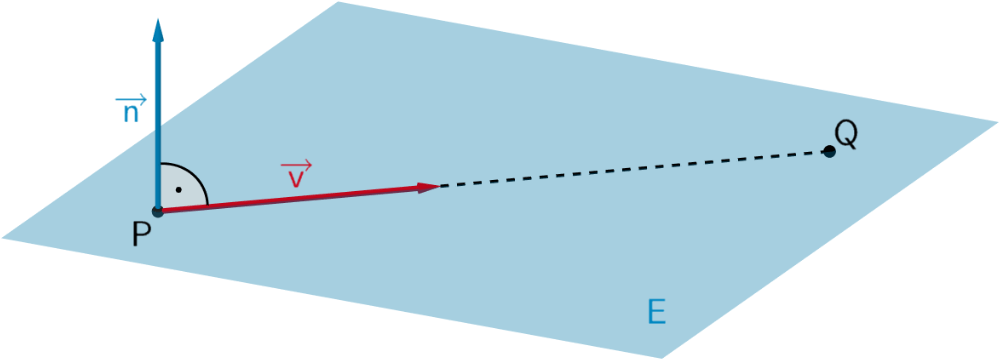
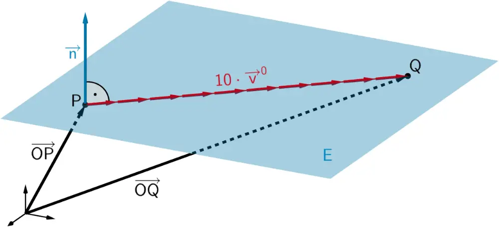
Planskizze (optional): Ausgehend von einem möglichen Punkt \(P\), liegt ein möglicher Punkt \(Q\) im Abstand 10 in Richtung eines Vektors \(\textcolor{#cc071e}{\overrightarrow{v}}\), der zum Nomalenvektor \(\textcolor{#0087c1}{\overrightarrow{n}}\) der Ebene \(\textcolor{#0087c1}{E}\) senkrecht ist.
Koordinaten eines möglichen Punktes \(\boldsymbol{P}\) bestimmen.
Am einfachsten ist es, für \(P\) einen Schnittpunkt der Ebene \(E\) mit einer Koordinatenachse zu wählen. Beispielsweise ist \(P(0|0|p_3)\) der Schnittpunkt der Ebene \(E\) mit der \(x_3\)-Achse.
\[\textcolor{#0087c1}{E} \colon 5x_1 - 4x_2 + 3x_3 - 6 = 0\]
\[\begin{align*}P(\textcolor{#e9b509}{0}|\textcolor{#e9b509}{0}|\textcolor{#e9b509}{p_3}) \in \textcolor{#0087c1}{E} \colon 5 \cdot \textcolor{#e9b509}{0} - 4 \cdot \textcolor{#e9b509}{0} + 3 \cdot \textcolor{#e9b509}{p_3} - 6 &= 0 &&| + 6 \\[0.8em] 3p_3 &= 6 &&| : 3 \\[0.8em] p_3 &= 2 \end{align*}\]
\[\Rightarrow P(0|0|2)\]
Vektor \(\boldsymbol{\textcolor{#cc071e}{\overrightarrow{v}}}\) bestimmen, der senkrecht zum Normalenvektor \(\boldsymbol{\textcolor{#0087c1}{\overrightarrow{n}}}\) ist.
Hierfür wird entweder das Vektorprodukt aus dem Normalenvektor \(\textcolor{#0087c1}{\overrightarrow{n}}\) und einem beliebigen Vektor \(\overrightarrow{u}\) angewendet oder durch „systematisches Probieren" ein geeigneter Vektor \(\textcolor{#cc071e}{\overrightarrow{v}}\) ermittelt, der die Bedingung \(\textcolor{#0087c1}{\overrightarrow{n}} \circ \textcolor{#cc071e}{\overrightarrow{v}} = 0 \Leftrightarrow \textcolor{#0087c1}{\overrightarrow{n}} \perp \textcolor{#cc071e}{\overrightarrow{v}}\) erfüllt.
Ebenengleichung in Normalenform
Jede Ebene lässt sich durch eine Gleichung in Normalenform beschreiben. Ist \(\textcolor{#0087c1}{A}\) ein beliebiger Aufpunkt der Ebene \(\textcolor{#0087c1}{E}\) und \(\textcolor{#e9b509}{\overrightarrow{n}}\) ein Normalenvektor von \(E\), so erfüllt jeder Punkt \(X\) der Ebene \(E\) folgende Gleichungen:

Normalenform in Vektordarstellung
\[E \colon \textcolor{#e9b509}{\overrightarrow{n}} \circ (\overrightarrow{OX} - \textcolor{#0087c1}{\overrightarrow{OA}}) = 0\]
Normalenform in Koordinatendarstellung
\[E \colon \textcolor{#e9b509}{n_{1}}x_{1} + \textcolor{#e9b509}{n_{2}}x_{2} + \textcolor{#e9b509}{n_{3}}x_{3} + k = 0\]
mit \(k = -(\overrightarrow{n} \circ \overrightarrow{OA}) = - n_{1}a_{1} - n_{2}a_{2} - n_{3}a_{3}\)
\(n_{1}\), \(n_{2}\) und \(n_{3}\): Koordinaten eines Normalenvektors \(\overrightarrow{n}\)
Sind zwei linear unabhängige Richtungsvektoren \(\textcolor{#cc071e}{\overrightarrow{u}}\) und \(\textcolor{#cc071e}{\overrightarrow{v}}\) einer Ebene \(E\) bekannt, liefert das Vektorprodukt \(\textcolor{#cc071e}{\overrightarrow{u}} \times \textcolor{#cc071e}{\overrightarrow{v}}\) einen Normalenvektor \(\textcolor{#e9b509}{\overrightarrow{n}}\) der Ebene \(E\).
\[\textcolor{#0087c1}{E} \colon \textcolor{#0087c1}{5}x_1 \textcolor{#0087c1}{- 4}x_2 + \textcolor{#0087c1}{3}x_3 - 6 = 0 \; \Rightarrow \; \textcolor{#0087c1}{\overrightarrow{n} = \begin{pmatrix} 5\\-4\\3 \end{pmatrix}}\]
Mithilfe des Vektorprodukts:
Das Vektorprodukt \(\textcolor{#0087c1}{\overrightarrow{n}} \times \overrightarrow{u}\) aus dem Normalenvektor \(\textcolor{#0087c1}{\overrightarrow{n}}\) und beispielsweise \(\overrightarrow{u} = \begin{pmatrix} 1\\0\\0 \end{pmatrix}\) ergibt einen Vektor \(\textcolor{#cc071e}{\overrightarrow{v}}\), der sowohl zu \(\textcolor{#0087c1}{\overrightarrow{n}}\) als auch zu \(\overrightarrow{u}\) senkrecht ist.
Vektorprodukt (Kreuzprodukt)
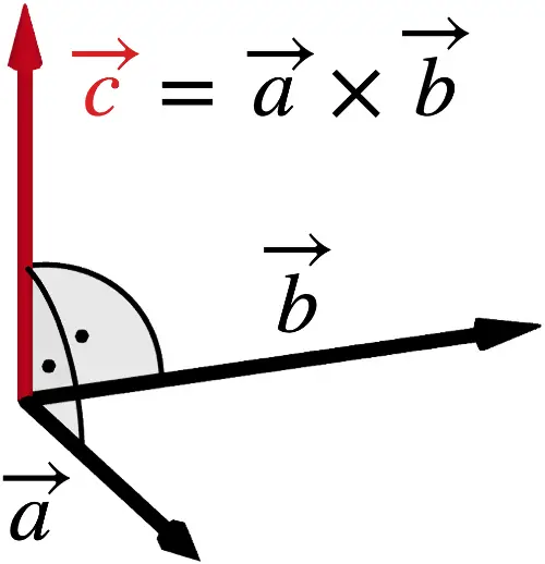
Das Vektorprodukt \(\overrightarrow{a} \times \overrightarrow{b}\) zweier Vektoren \(\overrightarrow{a}\neq \overrightarrow{0}\) und \(\overrightarrow{b} \neq \overrightarrow{0}\), die nicht parallel zueinander sind, erzeugt einen neuen Vektor \(\overrightarrow{c} = \overrightarrow{a} \times \overrightarrow{b}\), der zu beiden Vektoren \(\overrightarrow{a}\) und \(\overrightarrow{b}\) orthogonal (senkrecht) ist.
\[\textcolor{#cc071e}{\overrightarrow{c}} = \overrightarrow{a} \times \overrightarrow{b} \, \Rightarrow \begin{cases}\textcolor{#cc071e}{\overrightarrow{c}} \circ \overrightarrow{a} = 0\; \Leftrightarrow \;\textcolor{#cc071e}{\overrightarrow{c}} \perp \overrightarrow{a} \\\textcolor{#cc071e}{\overrightarrow{c}} \circ \overrightarrow{b} = 0\; \Leftrightarrow \;\textcolor{#cc071e}{\overrightarrow{c}} \perp \overrightarrow{b}\end{cases} \quad (\overrightarrow{a} \neq \overrightarrow{0},\, \overrightarrow{b} \neq \overrightarrow{0},\, \overrightarrow{a} \neq k \cdot \overrightarrow{b}\;\text{mit} \;k \in \mathbb R \backslash \{0\})\]
Es gilt: \(\overrightarrow{a} \times \overrightarrow{b} = \begin {pmatrix} a_1 \\ a_2 \\ a_3 \end {pmatrix} \times \begin {pmatrix} b_1 \\ b_2 \\ b_3 \end {pmatrix} = \begin {pmatrix} a_2 \cdot b_3 - a_3 \cdot b_2 \\ a_3 \cdot b_1 - a_1 \cdot b_3 \\ a_1 \cdot b_2 - a_2 \cdot b_1 \end {pmatrix}\)
\(\overrightarrow{a} \times \overrightarrow{b} = -\left(\overrightarrow{b} \times \overrightarrow{a}\right)\)
(Das Kommutativgesetz gilt nicht.)
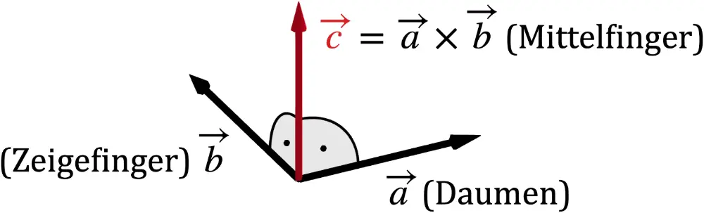
Die Rechte-Hand-Regel beschreibt die gegenseitige Lage der Vektoren \(\overrightarrow{a}\), \(\overrightarrow{b}\) und \(\textcolor{#cc071e}{\overrightarrow{c}} = \overrightarrow{a} \times \overrightarrow{b}\) im Raum. Weist \(\overrightarrow{a}\) in Richtung des Daumens und \(\overrightarrow{b}\) in Richtung des Zeigefingers, so weist der Mittelfinger in Richtung von \(\textcolor{#cc071e}{\overrightarrow{c}} = \overrightarrow{a} \times \overrightarrow{b}\).
\[\begin{align*} \textcolor{#cc071e}{\overrightarrow{v}} &= \textcolor{#0087c1}{\overrightarrow{n}} \times \overrightarrow{u} = \textcolor{#0087c1}{\begin{pmatrix} 5\\-4\\3 \end{pmatrix}} \times \begin{pmatrix} 1\\0\\0 \end{pmatrix} \\[0.8em] &= \begin{pmatrix} -4 & \cdot & 0 & - & 3 & \cdot & 0\\3 & \cdot & 1 & - & 5 & \cdot & 0 \\ 5 & \cdot & 0 & - & (-4) & \cdot & 1 \end{pmatrix}\\[0.8em] &= \textcolor{#cc071e}{\begin{pmatrix} 0\\3\\4 \end{pmatrix}} \end{align*}\]
Mithilfe des Skalarprodukts:
Für eine Koordinate von \(\textcolor{#cc071e}{\overrightarrow{v}}\) null wählen, beispielsweise \(\textcolor{#cc071e}{v_1 = 0}\). Für die anderen beiden Koordinaten \(\textcolor{#cc071e}{v_2}\) und \(\textcolor{#cc071e}{v_3}\) die Werte der Koordinaten \(\textcolor{#0087c1}{n_2}\) und \(\textcolor{#0087c1}{n_3}\) vertauschen und einmal das Vorzeichen wechseln. Also beispielsweise: \(\textcolor{#cc071e}{v_2} = \textcolor{#0087c1}{n_3}\) und \(\textcolor{#cc071e}{v_3} = \textcolor{#0087c1}{-n_2}\).
Anwendung des Skalarprodukts
Zueinander senkrechte (orthogonale) Vektoren
Zwei vom Nullvektor verschiedene Vektoren \(\overrightarrow{a}\) und \(\overrightarrow{b}\) sind genau dann zueinander senkrecht (orthogonal), wenn deren Skalarprodukt null ist.
\[\textcolor{#cc071e}{\overrightarrow{a}} \circ \textcolor{#0087c1}{\overrightarrow{b}} = 0 \; \Leftrightarrow \; \textcolor{#cc071e}{\overrightarrow{a}} \perp \textcolor{#0087c1}{\overrightarrow{b}}\]
\[\begin{align*}\textcolor{#0087c1}{\overrightarrow{n}} \circ \textcolor{#cc071e}{\overrightarrow{v}} &= 0 \\[0.8em] \textcolor{#0087c1}{\begin{pmatrix} 5 \\ -4 \\ 3 \end{pmatrix}} \circ \textcolor{#cc071e}{\begin{pmatrix} v_1\\v_2\\v_3 \end{pmatrix}} &= 0 \\[0.8em] \textcolor{#0087c1}{\begin{pmatrix} 5 \\ -4 \\ 3 \end{pmatrix}} \circ \textcolor{#cc071e}{\begin{pmatrix} 0\\3\\4 \end{pmatrix}} &= 0 \\[0.8em] 5 \cdot 0 - 4 \cdot 3 + 3 \cdot 4 &= 0 \\[0.8em] \Rightarrow \;\textcolor{#0087c1}{\overrightarrow{n}} \perp \textcolor{#cc071e}{\overrightarrow{v}} \end{align*}\]
Koordinaten eines möglichen Punktes \(\boldsymbol{Q}\) bestimmen.
Ein möglicher Punkt \(Q\) liegt im Abstand 10 von Punkt \(P(0|0|2)\) in Richtung des Vektors \(\textcolor{#cc071e}{\overrightarrow{v}}\).
1. Möglichkeit: Mithilfe des Einheitsvektors von \(\textcolor{#cc071e}{\overrightarrow{\boldsymbol{v}}}\)
Der Einheitsvektor \(\textcolor{#cc071e}{{\overrightarrow{v}}^0}\) des Vektors \(\textcolor{#cc071e}{\overrightarrow{v}}\) hat die Länge eins. Durch Vektoraddition ergibt sich:
Einheitsvektor
Ein Vektor mit dem Betrag 1 heißt Einheitsvektor. Mit Ausnahme des Nullvektors lässt sich jeder Vektor zu einem Einheitsvektor skalieren. Der zu einem Vektor \(\overrightarrow{a}\) gehörende Einheitsvektor wird mit \(\overrightarrow{a}^0\) bezeichnet.
Für \(\overrightarrow{a} \neq \overrightarrow{0}\) gilt: \(\overrightarrow{a}^{0} = \dfrac{\overrightarrow{a}}{\vert \overrightarrow{a}\vert}\) mit \(\vert\overrightarrow{a}^{0}\vert = \left|\dfrac{\overrightarrow{a}}{\vert \overrightarrow{a}\vert}\right| = 1\)
\[\begin{align*}\overrightarrow{OQ} &= \overrightarrow{OP} + \textcolor{#cc071e}{10 \cdot \overrightarrow{v}^0}= \overrightarrow{OP} + \textcolor{#cc071e}{10 \cdot \frac{\overrightarrow{v}}{\vert \overrightarrow{v} \vert}} \\[0.8em] &= \begin{pmatrix} 0\\0\\2 \end{pmatrix} + \textcolor{#cc071e}{10 \cdot \frac{\begin{pmatrix} 0\\3\\4 \end{pmatrix}}{\left|\begin{pmatrix} 0\\3\\4 \end{pmatrix}\right|}} = \begin{pmatrix} 0\\0\\2 \end{pmatrix} + 10 \cdot \frac{\begin{pmatrix} 0\\3\\4 \end{pmatrix}}{\sqrt{0^2+3^2+4^2}} \\[0.8em] &= \begin{pmatrix} 0\\0\\2 \end{pmatrix} + 10 \cdot \frac{\begin{pmatrix} 0\\3\\4 \end{pmatrix}}{5} = \begin{pmatrix} 0\\0\\2 \end{pmatrix} + 2 \cdot \begin{pmatrix} 0\\3\\4 \end{pmatrix} \\[0.8em]&= \begin{pmatrix} 0\\6\\10 \end{pmatrix} \; \Rightarrow \; Q(0|6|10)\end{align*}\]
Die Punkte \(P(0|0|2)\) und \(Q(0|6|10)\) liegen in der Ebene \(E\colon 5x_1 - 4x_2 + 3x_3 - 6 = 0\) und haben voneinander den Abstand 10.
(Vgl. Mathematik Abiturskript Bayern G9 - 3 Geometrie, 3.2.1 Rechnen mit Vektoren - Einheitsvektor)
2. Möglichkeit: Bedingung \(\boldsymbol{\vert \overrightarrow{PQ}\vert = \vert \textcolor{#cc071e}{\lambda \cdot \overrightarrow{v}}\vert = 10}\)

\(\overrightarrow{OQ} = \overrightarrow{OP} + \textcolor{#cc071e}{\lambda \cdot \overrightarrow{v}}\) mit \(\vert \textcolor{#cc071e}{\lambda \cdot \overrightarrow{v}}\vert = 10\)
Der Betrag eines Vektors \(\overrightarrow{a}\) bedeutet die Länge eines zu \(\overrightarrow{a}\) gehörenden Repräsentanten. Schreibweise: \(\vert \overrightarrow{a}\vert\)
Für \(\smash{\overrightarrow{a} = \begin{pmatrix} a_1\\a_2 \end{pmatrix}}\vphantom{\begin{pmatrix} a_1\\a_2\\a_3 \end{pmatrix}}\) gilt \(\vert \overrightarrow{a}\vert = \sqrt{a_1^2 + a_2^2}\)
Für \(\overrightarrow{a} = \begin{pmatrix} a_1\\a_2\\a_3 \end{pmatrix}\) gilt \(\vert \overrightarrow{a}\vert = \sqrt{a_1^2 + a_2^2 + a_3^2}\)
\[\begin{align*}\vert \textcolor{#cc071e}{\lambda \cdot \overrightarrow{v}}\vert &= 10 \\[0.8em] \left| \lambda \cdot \textcolor{#cc071e}{\begin{pmatrix} 0\\3\\4 \end{pmatrix}}\right| &= 10 \\[0.8em] \left| \begin{pmatrix} 0\\3\lambda \\4\lambda \end{pmatrix} \right| &= 10 \\[0.8em] \sqrt{0^2 +(3\lambda)^2 + (4\lambda)^2} &= 10 \\[0.8em] \sqrt{9\lambda^2 + 16\lambda^2} &= 0 \\[0.8em] \sqrt{25\lambda^2} &= 10 \\[0.8em] \sqrt{25} \cdot \sqrt{\lambda^2} &= 10 \\[0.8em] 5 \cdot \vert \lambda \vert &= 10 &&| :5 \\[0.8em] \vert \lambda \vert &= 2 \\[0.8em] \textcolor{#cc071e}{\lambda = 2} \; \vee \; \textcolor{#cc071e}{\lambda} &\;\textcolor{#cc071e}{= -2}\end{align*}\]
Koordinaten der möglichen Punkte \(Q\) berechnen:
\[\overrightarrow{OQ_1} = \begin{pmatrix} 0\\0\\2 \end{pmatrix} + \textcolor{#cc071e}{2 \cdot \begin{pmatrix} 0\\3\\4 \end{pmatrix}} = \begin{pmatrix} 0\\6\\10 \end{pmatrix}\; \Rightarrow \; Q_1(0|6|10)\]
\[\overrightarrow{OQ_2} = \begin{pmatrix} 0\\0\\2 \end{pmatrix} + \textcolor{#cc071e}{(-2) \cdot \begin{pmatrix} 0\\3\\4 \end{pmatrix}} = \begin{pmatrix} 0\\-6\\-6 \end{pmatrix}\; \Rightarrow \; Q_2(0|-6|-6)\]
Die Punkte \(P(0|0|2)\) und \(Q_1(0|6|10)\) bzw. \(Q_2(0|-6|-6)\) liegen in der Ebene \(E\colon 5x_1 - 4x_2 + 3x_3 - 6 = 0\) und haben voneinander den Abstand 10.
(Vgl. Mathematik Abiturskript Bayern G9 - 3 Geometrie, 3.2.1 Rechnen mit Vektoren - Betrag eines Vektors)