Bestimmen Sie eine Gleichung von \(L\) in Koordinatenform sowie die Größe \(\varphi\) des Winkels, den \(L\) mit der \(x_1x_2\)-Ebene einschließt.
(zur Kontrolle: \(x_1+x_2+x_3-19= 0; \enspace \varphi \approx 55^{\circ}\))
(6 BE)
Lösung zu Teilaufgabe b
Gleichung der Ebene \(L\) in Koordinatenform
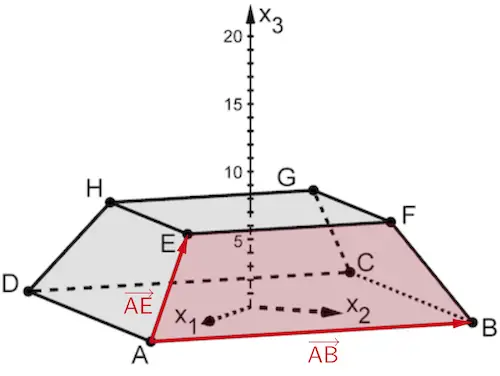 Abb. 1
Das Trapez \(ABFE\) liegt in der Ebene \(L\). Beispielsweise liefert das Vektorprodukt \(\textcolor{#cc071e}{\overrightarrow{AB} \times \overrightarrow{AE}}\) der beiden linear unabhängigen Verbindungsvektoren \(\textcolor{#cc071e}{\overrightarrow{AB}}\) und \(\textcolor{#cc071e}{\overrightarrow{AE}}\) einen Normalenvektor der Ebene \(L\). Als Aufpunkt wählt man einen der Punkte \(A\), \(B\), \(F\) oder \(E\). Damit lässt sich eine Gleichung der Ebene \(L\) in Koordinatenform (Normalenform in Koordinatendarstellung) bestimmen.
Lineare (Un)Abhängigkeit von zwei Vektoren
Zwei Vektoren \(\overrightarrow{a}\) und \(\overrightarrow{b}\) sind
linear abhängig, wenn
\(\overrightarrow{a} \parallel \overrightarrow{b}\) bzw. \(\overrightarrow{a} = k \cdot \overrightarrow{b}\) mit \(k \in \mathbb R\) gilt.
linear unabhängig, wenn
\(\overrightarrow{a} \nparallel \overrightarrow{b}\) bzw. \(\overrightarrow{a} \neq k \cdot \overrightarrow{b}\) mit \(k \in \mathbb R\) gilt.
Lineare (Un-)Abhängigkeit von drei Vektoren
Drei Vektoren \(\overrightarrow{a}\), \(\overrightarrow{b}\) und \(\overrightarrow{c}\) sind
linear abhängig, wenn
sie in einer Ebene liegen bzw. wenn beispielsweise
die lineare Vektorgleichung \(\overrightarrow{c} = r \cdot \overrightarrow{a} + s \cdot \overrightarrow{b}\) eine eindeutige Lösung hat.
linear unabhängig, wenn
sie den Raum \(\mathbb R^{3}\) aufspannen bzw. wenn beispielsweise
die lineare Vektorgleichung \(\overrightarrow{c} = r \cdot \overrightarrow{a} + s \cdot \overrightarrow{b}\) keine Lösung hat.
Der Ansatz kann mithilfe der Normalenform in Vektordarstellung oder in Koordinatendarstellung erfolgen.
Ebenengleichung in Normalenform (vgl. Merkhilfe)
Jede Ebene lässt sich durch eine Gleichung in Normalenform beschreiben. Ist \(A\) ein beliebiger Aufpunkt der Ebene \(E\) und \(\overrightarrow{n}_{E}\) ein Normalenvektor von \(E\), so erfüllt jeder Punkt \(X\) der Ebene \(E\) folgende Gleichungen:
Normalenform in Vektordarstellung
\[E \colon \overrightarrow{n}_{E} \circ (\overrightarrow{X} - \overrightarrow{A}) = 0\]

Normalenform in Koordinatendarstellung
\[E \colon n_{1}x_{1} + n_{2}x_{2} + n_{3}x_{3} + n_{0} = 0\]
mit \(n_{0} = -(\overrightarrow{n}_{E} \circ \overrightarrow{A}) = - \: n_{1}a_{1} - n_{2}a_{2} - n_{3}a_{3}\)
\(n_{1}\), \(n_{2}\) und \(n_{3}\): Koordinaten eines Normalenvektors \(\overrightarrow{n}_{E}\)
Die Verbindungsvektoren \(\textcolor{#cc071e}{\overrightarrow{AB}}\) und \(\textcolor{#cc071e}{\overrightarrow{AE}}\) sollten aus Teilaufgabe a bekannt sein.
\(\textcolor{#cc071e}{\overrightarrow{AB}} = \textcolor{#cc071e}{\begin{pmatrix} -19 \\ 19 \\ 0 \end{pmatrix}}\); \(\textcolor{#cc071e}{\overrightarrow{AE}} = \textcolor{#cc071e}{\begin{pmatrix} -7 \\ 0 \\ 7 \end{pmatrix}}\)
Normalenvektor \(\textcolor{#0087c1}{\overrightarrow{n}}\) der Ebene \(L\) ermitteln:
Vektorprodukt (Kreuzprodukt)
Das Vektorprodukt \(\overrightarrow{a} \times \overrightarrow{b}\) zweier Vektoren \(\overrightarrow{a}\) und \(\overrightarrow{b}\) erzeugt einen neuen Vektor \(\overrightarrow{c} = \overrightarrow{a} \times \overrightarrow{b}\) mit den Eigenschaften:
\(\overrightarrow{c}\) ist sowohl zu \(\overrightarrow{a}\) als auch zu \(\overrightarrow{b}\) senkrecht.
\[\overrightarrow{c} = \overrightarrow{a} \times \overrightarrow{b} \quad \Longrightarrow \quad \overrightarrow{c} \perp \overrightarrow{a}, \enspace \overrightarrow{c} \perp \overrightarrow{b}\]
Der Betrag des Vektorprodukts zweier Vektoren \(\overrightarrow{a}\) und \(\overrightarrow{b}\) ist gleich dem Produkt aus den Beträgen der Vektoren \(\overrightarrow{a}\) und \(\overrightarrow{b}\) und dem Sinus des von ihnen eingeschlossenen Winkels \(\varphi\).
\[\vert \overrightarrow{a} \times \overrightarrow{b} \vert = \vert \overrightarrow{a} \vert \cdot \vert \overrightarrow{b} \vert \cdot \sin{\varphi} \quad (0^{\circ} \leq \varphi \leq 180^{\circ})\]
Die Vektoren \(\overrightarrow{a}\), \(\overrightarrow{b}\) und \(\overrightarrow{c}\) bilden in dieser Reihenfolge ein Rechtssystem. Rechtehandregel: Weist \(\overrightarrow{a}\) in Richtung des Daumens und \(\overrightarrow{b}\) in Richtung des Zeigefingers, dann weist \(\overrightarrow{c} = \overrightarrow{a} \times \overrightarrow{b}\) in Richtung des Mittelfingers.
Berechnung eines Vektorprodukts im \(\boldsymbol{\mathbb R^{3}}\) (vgl. Merkhilfe)
\[\overrightarrow{a} \times \overrightarrow{b} = \begin {pmatrix} a_1 \\ a_2 \\ a_3 \end {pmatrix} \times \begin {pmatrix} b_1 \\ b_2 \\ b_3 \end {pmatrix} = \begin {pmatrix} a_2 \cdot b_3 - a_3 \cdot b_2 \\ a_3 \cdot b_1 - a_1 \cdot b_3 \\ a_1 \cdot b_2 - a_2 \cdot b_1 \end {pmatrix}\]
\[\begin{align*} \textcolor{#cc071e}{\overrightarrow{AB}} \times \textcolor{#cc071e}{\overrightarrow{AE}} &= \textcolor{#cc071e}{\begin{pmatrix} -19 \\ 19 \\ 0 \end{pmatrix}} \times \textcolor{#cc071e}{\begin{pmatrix} -7 \\ 0 \\ 7 \end{pmatrix}} \\[0.8em] &= \begin{pmatrix} 19 & \cdot & 7 & - & 0 & \cdot & 0 \\ 0 & \cdot & (-7) & - & (-19) & \cdot & 7 \\ -19 & \cdot & 0 & - & 19 & \cdot & (-7) \end{pmatrix} \\[0.8em] &= 19 \cdot 7 \cdot \begin{pmatrix} 1 \\ 1 \\ 1 \end{pmatrix} \end{align*}\]
Somit ist der Vektor \(\textcolor{#0087c1}{\overrightarrow{n} = \begin{pmatrix} 1 \\ 1 \\ 1 \end{pmatrix}}\) ein Normalenvektor der Ebene \(L\).
Gleichung der Ebene \(L\) in Koordinatenform bestimmen:
Der Punkt \(\textcolor{#e9b509}{A(19|0|0)}\) dient beispielsweise als Aufpunkt.
1. Möglichkeit: Ansatz mit Normalenform in Vektordarstellung
Ebenengleichung in Normalenform (vgl. Merkhilfe)
Jede Ebene lässt sich durch eine Gleichung in Normalenform beschreiben. Ist \(A\) ein beliebiger Aufpunkt der Ebene \(E\) und \(\overrightarrow{n}_{E}\) ein Normalenvektor von \(E\), so erfüllt jeder Punkt \(X\) der Ebene \(E\) folgende Gleichungen:
Normalenform in Vektordarstellung
\[E \colon \overrightarrow{n}_{E} \circ (\overrightarrow{X} - \overrightarrow{A}) = 0\]
Normalenform in Koordinatendarstellung
\[E \colon n_{1}x_{1} + n_{2}x_{2} + n_{3}x_{3} + n_{0} = 0\]
mit \(n_{0} = -(\overrightarrow{n}_{E} \circ \overrightarrow{A}) = - \: n_{1}a_{1} - n_{2}a_{2} - n_{3}a_{3}\)
\(n_{1}\), \(n_{2}\) und \(n_{3}\): Koordinaten eines Normalenvektors \(\overrightarrow{n}_{E}\)
\[\begin{align*}L \colon &\,\textcolor{#0087c1}{\overrightarrow{n}} \circ (\overrightarrow{X} - \textcolor{#e9b509}{\overrightarrow{A})} = 0 \\[0.8em] L \colon &\textcolor{#0087c1}{\begin{pmatrix} 1 \\ 1 \\ 1 \end{pmatrix}} \circ \left[ \overrightarrow{X} - \textcolor{#e9b509}{\begin{pmatrix} 19 \\ 0 \\ 0 \end{pmatrix}} \right] = 0 \\[0.8em] &\,\textcolor{#0087c1}{1} \cdot (x_{1} - \textcolor{#e9b509}{19}) + \textcolor{#0087c1}{1} \cdot (x_{2} - \textcolor{#e9b509}{0}) + \textcolor{#0087c1}{1} \cdot (x_{3} - \textcolor{#e9b509}{0}) = 0 \\[0.8em] &\,x_1 - 19 + x_2 + x_3 = 0 \\[0.8em] L \colon\, &x_{1} + x_{2} + x_{3} - 19 = 0 \end{align*}\]
2. Möglichkeit: Ansatz mit Normalenform in Koordinatendarstellung
\(\textcolor{#0087c1}{\overrightarrow{n} = \begin{pmatrix} 1 \\ 1 \\ 1 \end{pmatrix}}\); \(\textcolor{#e9b509}{A(19|0|0)}\)
Ebenengleichung in Normalenform (vgl. Merkhilfe)
Jede Ebene lässt sich durch eine Gleichung in Normalenform beschreiben. Ist \(A\) ein beliebiger Aufpunkt der Ebene \(E\) und \(\overrightarrow{n}_{E}\) ein Normalenvektor von \(E\), so erfüllt jeder Punkt \(X\) der Ebene \(E\) folgende Gleichungen:
Normalenform in Vektordarstellung
\[E \colon \overrightarrow{n}_{E} \circ (\overrightarrow{X} - \overrightarrow{A}) = 0\]
Normalenform in Koordinatendarstellung
\[E \colon n_{1}x_{1} + n_{2}x_{2} + n_{3}x_{3} + n_{0} = 0\]
mit \(n_{0} = -(\overrightarrow{n}_{E} \circ \overrightarrow{A}) = - \: n_{1}a_{1} - n_{2}a_{2} - n_{3}a_{3}\)
\(n_{1}\), \(n_{2}\) und \(n_{3}\): Koordinaten eines Normalenvektors \(\overrightarrow{n}_{E}\)
\[\begin{align*} &L \colon n_{1}x_{1} + n_{2}x_{2} + n_{3}x_{3} + n_{0} = 0 \\[0.8em] &L \colon \textcolor{#0087c1}{1} \cdot x_{1} + \textcolor{#0087c1}{1} \cdot x_{2} + \textcolor{#0087c1}{1} \cdot x_{3} + n_{0} = 0\\[0.8em] &L\colon x_{1} + x_{2} + x_{3} + n_{0} = 0 \end{align*}\]
\[\begin{align*} \textcolor{#e9b509}{A} \in L \colon \textcolor{#e9b509}{19} + \textcolor{#e9b509}{0} + \textcolor{#e9b509}{0} + n_{0} &= 0 &&| - 19 \\[0.8em] n_{0} &= 19 \end{align*}\]
\[\Rightarrow \enspace L \colon x_{1} + x_{2} + x_{3} - 19 = 0\]
Größe \(\varphi\) des Winkels, den \(L\) mit der \(x_1x_2\)-Ebene einschließt
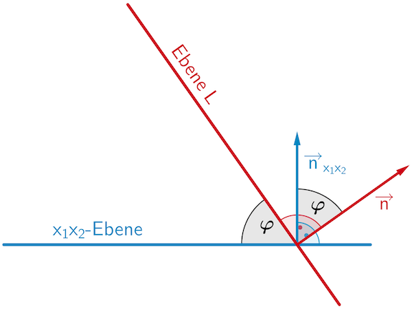
Der Winkel, den die Ebene \(\textcolor{#cc071e}{L}\) mit der \(\textcolor{#0087c1}{x_1x_2}\)-Ebene einschließt (Schnittwinkel), ist gleich dem Winkel zwischen den Normalenvektoren der Ebenen (Skizze schematisch, nicht verlangt).
\(\textcolor{#0087c1}{\overrightarrow{n}_{x_1x_2} = \begin{pmatrix} 0 \\ 0 \\ 1 \end{pmatrix}}\) ist ein Normalenvektor der \(\textcolor{#0087c1}{x_1x_2}\)-Ebene.
\(\textcolor{#cc071e}{\overrightarrow{n} = \begin{pmatrix} 1 \\ 1 \\ 1 \end{pmatrix}}\) ist ein Normalenvektor der Ebene \(\textcolor{#cc071e}{L}\).
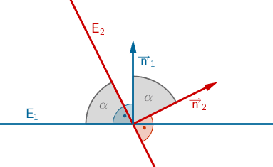
Schnittwinkel \(\boldsymbol{\alpha}\) zweier Ebenen
\[E_1\colon \enspace \overrightarrow{n}_1 \circ \left( \overrightarrow{X} - \overrightarrow{A} \right) = 0\]
\[E_2\colon \enspace \overrightarrow{n}_2 \circ \left( \overrightarrow{X} - \overrightarrow{B} \right) = 0\]
\[\cos \alpha = \frac{\vert \overrightarrow{n}_1 \circ \overrightarrow{n}_2 \vert}{\vert \overrightarrow{n}_1 \vert \cdot \vert \overrightarrow{n}_2 \vert} \enspace \Rightarrow \enspace \alpha = \cos^{-1}(\dots)\]
\[(0^{\circ} \leq \alpha \leq 90^{\circ})\]
\[\begin{align*} \cos{\varphi} &= \frac{\vert \textcolor{#cc071e}{\overrightarrow{n}} \circ \textcolor{#0087c1}{\overrightarrow{n}_{x_1x_2}} \vert}{\vert \textcolor{#cc071e}{\overrightarrow{n}} \vert \cdot \vert \textcolor{#0087c1}{\overrightarrow{n}_{x_1x_2}} \vert} = \frac{\left| \textcolor{#cc071e}{\begin{pmatrix} 1 \\ 1 \\ 1 \end{pmatrix}} \circ \textcolor{#0087c1}{\begin{pmatrix} 0 \\ 0 \\ 1 \end{pmatrix}} \right|}{\left| \textcolor{#cc071e}{\begin{pmatrix} 1 \\ 1 \\ 1 \end{pmatrix}} \right| \cdot \left| \textcolor{#0087c1}{\begin{pmatrix} 0 \\ 0 \\ 1 \end{pmatrix}} \right|} \\[0.8em] &= \frac{\vert \textcolor{#cc071e}{1} \cdot \textcolor{#0087c1}{0} + \textcolor{#cc071e}{1} \cdot \textcolor{#0087c1}{0} + \textcolor{#cc071e}{1} \cdot \textcolor{#0087c1}{1} \vert}{\sqrt{\textcolor{#cc071e}{1}^2 + \textcolor{#cc071e}{1}^2 + \textcolor{#cc071e}{1}^2} \cdot \sqrt{\textcolor{#0087c1}{0}^2 + \textcolor{#0087c1}{0}^2 + \textcolor{#0087c1}{1}^2}} \\[0.8em] &= \frac{1}{\sqrt{3}} &&| \; \text{TR:}\; \cos^{-1}(\dots) \\[2.4em] \varphi &= \cos^{-1}\left( \frac{1}{\sqrt{3}} \right) \approx 54{,}7^{\circ}\end{align*}\]
Die Größe \(\varphi\) des Winkels, den \(L\) mit der \(x_1x_2\)-Ebene einschließt, beträgt etwa 55° (vgl. Kontrollergebnis).