Ein Fotograf soll für ein Reisemagazin Unterwasserfotos aufnehmen.
Der Fotograf schwimmt entlang der kürzestmöglichen Strecke von der Uferlinie aus zur Boje. Ermitteln Sie die Länge dieser Strecke.
(4 BE)
Lösung zu Teilaufgabe e
Die Aufgabe behandelt das Thema Abstand Punkt - Gerade
(vgl. ![]() Bestimmung des Abstands zwischen Punkt und Gerade - 3 Möglichkeiten, Abiturskript - 2.4.1 Abstand Punkt - Gerade)
Bestimmung des Abstands zwischen Punkt und Gerade - 3 Möglichkeiten, Abiturskript - 2.4.1 Abstand Punkt - Gerade)

Planskizze (optional): Im Modell entspricht die Länge der kürzestmögliche Strecke von der Uferlinie zur Boje dem Abstand des Koordinatenursprungs \(O\) von der Gerade \(g\). Dieser ist gleich der Länge des Ortsvektors \(\textcolor{#0087c1}{\overrightarrow{F}}\) des Lotfußpunktes \(F\) (Lot von \(O\) auf \(g\)).
\[d(O;g) = \vert \textcolor{#0087c1}{\overrightarrow{F}} \vert\]
Drei mögliche Lösungsansätze für die Bestimmung des Ortsvektors \(\textcolor{#0087c1}{\overrightarrow{F}}\):
1. Möglichkeit: Skalarprodukt orthogonaler Vektoren anwenden
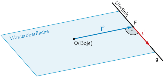
Planskizze (optional): Der Ortsvektor \(\textcolor{#0087c1}{\overrightarrow{F}}\) und der Richtungsvektor \(\textcolor{#cc071e}{\overrightarrow{u}}\) der Gerade \(g\) sind zueinander senkrecht (orthogonal). Folglich gilt:
\[g \colon \overrightarrow{X} = \begin{pmatrix} -12 \\ 11 \\ 0 \end{pmatrix} + \lambda \cdot \textcolor{#cc071e}{\begin{pmatrix} 1 \\ 2 \\ 0 \end{pmatrix}}, \; \lambda \in \mathbb R\]
Anwendung des Skalarprodukts:
Orthogonale (zueinander senkrechte) Vektoren (vgl. Merkhilfe)
\[\overrightarrow{a} \perp \overrightarrow{b} \; \Leftrightarrow \; \overrightarrow{a} \circ \overrightarrow{b} \quad (\overrightarrow{a} \neq \overrightarrow{0},\; \overrightarrow{b} \neq \overrightarrow{0})\]
\[\textcolor{#0087c1}{\overrightarrow{F}} \perp \textcolor{#cc071e}{\overrightarrow{u}} \enspace \Leftrightarrow \enspace \textcolor{#0087c1}{\overrightarrow{F}} \circ \textcolor{#cc071e}{\overrightarrow{u}} = 0\]
Zunächst wird der Ortsvektor \(\overrightarrow{F}\) in Abhängigkeit des Parameters \(\lambda\) der Gleichung der Gerade \(g\) formuliert.
\[\begin{align*}g \colon \overrightarrow{X} &= \begin{pmatrix} -12 \\ 11 \\ 0 \end{pmatrix} + \lambda \cdot \begin{pmatrix} 1 \\ 2 \\ 0 \end{pmatrix}, \; \lambda \in \mathbb R \\[0.8em]F \in g \colon \textcolor{#0087c1}{\overrightarrow{F}} &= \begin{pmatrix} -12 \\ 11 \\ 0 \end{pmatrix} + \lambda \cdot \begin{pmatrix} 1 \\ 2 \\ 0 \end{pmatrix} = \textcolor{#0087c1}{\begin{pmatrix} -12 + \lambda \\ 11 + 2\lambda \\ 0 \end{pmatrix}}, \; \lambda \in \mathbb R\end{align*}\]
Wendet man nun das Skalarprodukt der orthogonalen Vektoren \(\textcolor{#0087c1}{\overrightarrow{F}}\) und \(\textcolor{#cc071e}{\overrightarrow{u}}\) an, so liefert die Lösung der Gleichung denjenigen Wert des Parameters \(\lambda\), der eingesetzt in die Gleichung der Gerade \(g\) den Ortsvektor \(\textcolor{#0087c1}{\overrightarrow{F}}\) ergibt.
Skalarprodukt
Unter dem Skalarprodukt \(\overrightarrow{a} \circ \overrightarrow{b}\) zweier Vektoren \(\overrightarrow{a}\) und \(\overrightarrow{b}\) versteht man das Produkt aus den Beträgen der beiden Vektoren und dem Kosinus des von den Vektoren eingeschlossenen Winkels \(\varphi\).
\[\overrightarrow{a} \circ \overrightarrow{b} = \vert \overrightarrow{a} \vert \cdot \vert \overrightarrow{b} \vert \cdot \cos{\varphi} \quad (0^{\circ} \leq \varphi \leq 180^{\circ})\]
Berechnung eines Skalarprodukts im \(\boldsymbol{\mathbb R^{3}}\) (vgl. Merkhilfe)
\[\overrightarrow{a} \circ \overrightarrow{b} = \begin{pmatrix} a_{1} \\ a_{2} \\ a_{3} \end{pmatrix} \circ \begin{pmatrix} b_{1} \\ b_{2} \\ b_{3} \end{pmatrix} = a_{1}b_{1} + a_{2}b_{2} + a_{3}b_{3}\]
\[\begin{align*} \textcolor{#0087c1}{\begin{pmatrix} -12 + \lambda \\ 11 + 2\lambda \\ 0 \end{pmatrix}} \circ \textcolor{#cc071e}{\begin{pmatrix} 1 \\ 2 \\ 0 \end{pmatrix}} &= 0 \\[0.8em] \textcolor{#0087c1}{(-12 + \lambda)} \cdot \textcolor{#cc071e}{1} + \textcolor{#0087c1}{(11 + 2\lambda)} \cdot \textcolor{#cc071e}{2} + \textcolor{#0087c1}{0} \cdot \textcolor{#cc071e}{0} &= 0 \\[0.8em] -12 + \lambda + 22 + 4\lambda &= 0 \\[0.8em] 10 + 5\lambda &= 0 &&| -10 \\[0.8em] 5\lambda &= -10 &&| : 5 \\[0.8em] \lambda &= \textcolor{#e9b509}{-2}\end{align*}\]
\[\textcolor{#0087c1}{\overrightarrow{F}} = \textcolor{#0087c1}{\begin{pmatrix} -12 + \textcolor{#e9b509}{(-2)} \\ 11 + 2 \cdot \textcolor{#e9b509}{(-2)} \\ 0 \end{pmatrix}} = \textcolor{#0087c1}{\begin{pmatrix} -14 \\ 7 \\ 0 \end{pmatrix}}\]
Länge der kürzestmögliche Strecke von der Uferlinie zur Boje berechnen:
Betrag eines Vektors
\[ \vert \overrightarrow{a} \vert = \sqrt{\overrightarrow{a} \circ \overrightarrow{a}} = \sqrt{{a_1}^2 + {a_2}^2 + {a_3}^2}\]
(vgl. Merkhilfe)
\[\begin{align*}d(O;g) &= \vert \textcolor{#0087c1}{\overrightarrow{F}} \vert = \left| \textcolor{#0087c1}{\begin{pmatrix} -14 \\ 7 \\ 0 \end{pmatrix}} \right| = \sqrt{(-14)^2 + 7^2 + 0^2} \\[0.8em] &= \sqrt{245} = 7\sqrt{5} \approx 15{,}7\end{align*}\]
Der Fotograf schwimmt eine Strecke von knapp 16 m.
2. Möglichkeit: Hilfsebene aufstellen
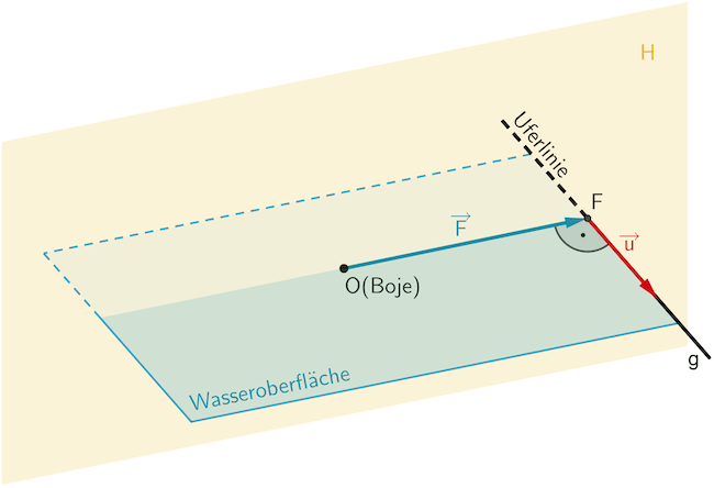
Planskizze (optional): Die Hilfsebene \(\textcolor{#e9b509}{H}\) mit den Eigenschaften \(O \in \textcolor{#e9b509}{H}\) und \(g \perp \textcolor{#e9b509}{H}\) schneidet die Gerade \(g\) im Lotfußpunkt \(F\) (Lot von \(O\) auf \(g\)).
Der Richtungsvektor \(\textcolor{#cc071e}{\overrightarrow{u} = \begin{pmatrix} 1 \\ 2 \\ 0 \end{pmatrix}}\) der Gerade \(g\) ist ein Normalenvektor der Hilfsebene \(\textcolor{#e9b509}{H}\). Der Koordinatenursprung \(O(0|0|0)\) dient als Aufpunkt für eine Gleichung von \(\textcolor{#e9b509}{H}\) in Normalenform.
Gleichung der Hilfsebene \(\textcolor{#e9b509}{H}\) in Normalenform in Koordinatendarstellung (Koordinatenform) aufstellen:
(Ansatz mit Vektordarstellung oder Koordinatendarstellung möglich)
Ebenengleichung in Normalenform (vgl. Merkhilfe)
Jede Ebene lässt sich durch eine Gleichung in Normalenform beschreiben. Ist \(A\) ein beliebiger Aufpunkt der Ebene \(E\) und \(\overrightarrow{n}_{E}\) ein Normalenvektor von \(E\), so erfüllt jeder Punkt \(X\) der Ebene \(E\) folgende Gleichungen:
Normalenform in Vektordarstellung
\[E \colon \overrightarrow{n}_{E} \circ (\overrightarrow{X} - \overrightarrow{A}) = 0\]

Normalenform in Koordinatendarstellung
\[E \colon n_{1}x_{1} + n_{2}x_{2} + n_{3}x_{3} + n_{0} = 0\]
mit \(n_{0} = -(\overrightarrow{n}_{E} \circ \overrightarrow{A}) = - \: n_{1}a_{1} - n_{2}a_{2} - n_{3}a_{3}\)
\(n_{1}\), \(n_{2}\) und \(n_{3}\): Koordinaten eines Normalenvektors \(\overrightarrow{n}_{E}\)
\[\begin{align*} \textcolor{#e9b509}{H} \colon \textcolor{#cc071e}{\overrightarrow{u}} \circ \Big( \overrightarrow{X} - \overrightarrow{O} \Big) &= 0 \\[0.8em] \textcolor{#cc071e}{\begin{pmatrix} 1 \\ 2 \\ 0 \end{pmatrix}} \circ \left[ \overrightarrow{X} - \begin{pmatrix} 0 \\ 0 \\ 0 \end{pmatrix} \right] &= 0 \\[0.8em] \textcolor{#cc071e}{1} \cdot x_{1} + \textcolor{#cc071e}{2} \cdot x_{2} + \textcolor{#cc071e}{0} \cdot x_{3} &= 0 \\[0.8em] \textcolor{#e9b509}{H} \colon x_{1} + 2x_{2} &= 0\end{align*}\]
oder
\[\begin{align*} \textcolor{#e9b509}{H} \colon \textcolor{#cc071e}{n_{1}}x_{1} + \textcolor{#cc071e}{n_{2}}x_{2} + \textcolor{#cc071e}{n_{3}}x_{3} + n_{0} &= 0 \\[0.8em] \textcolor{#cc071e}{1} \cdot x_{1} + \textcolor{#cc071e}{2} \cdot x_{2} + \textcolor{#cc071e}{0} \cdot x_{3} + n_{0} &= 0 \\[0.8em] x_{1} + 2x_{2} + n_{0} &= 0\end{align*}\]
\[\begin{align*}O(0|0|0) \in \textcolor{#e9b509}{H} \colon 0 + 2 \cdot 0 + n_{0} &= 0 \\[0.8em] n_{0} &= 0\end{align*}\]
\[\Rightarrow \enspace \textcolor{#e9b509}{H} \colon x_{1} + 2x_{2} = 0\]
Schnittpunkt \(F\) der Gerade \(g\) und der Hilfsebene \(\textcolor{#e9b509}{H}\) bestimmen:
Hierfür werden die Koordinaten der Gleichung der Gerade \(g\) in die Gleichung der Hilfsebene \(\textcolor{#e9b509}{H}\) eingesetzt und diese nach dem Parameter \(\lambda\) aufgelöst.
\[g \colon \overrightarrow{X} = \begin{pmatrix} -12 \\ 11 \\ 0 \end{pmatrix} + \lambda \cdot \begin{pmatrix} 1 \\ 2 \\ 0 \end{pmatrix} = \begin{pmatrix} -12 + \lambda \\ 11 + 2\lambda \\ 0 \end{pmatrix}, \; \lambda \in \mathbb R\]
\[\textcolor{#e9b509}{H} \colon x_{1} + 2x_{2} = 0\]
\[\begin{align*}g \cap \textcolor{#e9b509}{H}\colon -12 + \lambda + 2 \cdot (11 + 2\lambda) &= 0 \\[0.8em] -12 + \lambda +22 + 4\lambda &= 0 \\[0.8em] 10 + 5\lambda &= 0 &&| -10 \\[0.8em] 5\lambda &= -10 &&| : 5 \\[0.8em] \lambda &= \textcolor{#89ba17}{-2}\end{align*}\]
Durch Einsetzen des Parameterwerts \(\lambda = \textcolor{#89ba17}{-2}\) in die Gleichung der Gerade \(g\) erhält man den Ortsvektor \(\textcolor{#0087c1}{\overrightarrow{F}}\).
\[F \in g \colon \textcolor{#0087c1}{\overrightarrow{F}} = \begin{pmatrix} -12 + \textcolor{#89ba17}{(-2)}\\ 11 + 2 \cdot \textcolor{#89ba17}{(-2)} \\ 0 \end{pmatrix} = \textcolor{#0087c1}{\begin{pmatrix} -14 \\ 7 \\ 0 \end{pmatrix}}\]
Länge der kürzestmögliche Strecke von der Uferlinie zur Boje berechnen:
Betrag eines Vektors
\[ \vert \overrightarrow{a} \vert = \sqrt{\overrightarrow{a} \circ \overrightarrow{a}} = \sqrt{{a_1}^2 + {a_2}^2 + {a_3}^2}\]
(vgl. Merkhilfe)
\[\begin{align*}d(O;g) &= \vert \textcolor{#0087c1}{\overrightarrow{F}} \vert = \left| \textcolor{#0087c1}{\begin{pmatrix} -14 \\ 7 \\ 0 \end{pmatrix}} \right| = \sqrt{(-14)^2 + 7^2 + 0^2} \\[0.8em] &= \sqrt{245} = 7\sqrt{5} \approx 15{,}7\end{align*}\]
Der Fotograf schwimmt eine Strecke von knapp 16 m.
3. Möglichkeit: Differentialrechnung anwenden
![Länge der Strecke [OX] zwischen dem Koordinatenursprung O und einem beliebigen Punkt X ∈ g](/images/stories/B2022_PT_B_G1/B2022_PT_B_G1_e_4.png)
Planskizze (optional): Die Länge der Strecke \(\textcolor{#e9b509}{[OX]}\) zwischen dem Koordinatenursprung \(O\) und einem beliebigen Punkt \(X \in g\) lässt sich in Abhängigkeit des Parameters \(\lambda\) der Geradengleichung von \(g\) formulieren.
Die notwendige Bedingung für die kürzeste Strecke \(\textcolor{#e9b509}{[OX]}\) (Lot von \(O\) auf \(g\)) lautet \(\textcolor{#e9b509}{\overline{OX}'(\lambda) = 0}\). Die Lösung der Gleichung liefert denjenigen Wert des Parameters \(\lambda\), der eingesetzt in die Gleichung von \(g\) den Ortsvektor \(\textcolor{#0087c1}{\overrightarrow{F}}\) ergibt.
Ortsvektor \(\textcolor{#e9b509}{\overrightarrow{X}}\) in Abhängigkeit des Parameters \(\lambda\) der Gleichung der Gerade \(g\) formulieren:
\[\begin{align*}g \colon \overrightarrow{X} &= \begin{pmatrix} -12 \\ 11 \\ 0 \end{pmatrix} + \lambda \cdot \begin{pmatrix} 1 \\ 2 \\ 0 \end{pmatrix}, \; \lambda \in \mathbb R \\[0.8em]X \in g \colon \textcolor{#e9b509}{\overrightarrow{X}} &= \begin{pmatrix} -12 \\ 11 \\ 0 \end{pmatrix} + \lambda \cdot \begin{pmatrix} 1 \\ 2 \\ 0 \end{pmatrix} = \textcolor{#e9b509}{\begin{pmatrix} -12 + \lambda \\ 11 + 2\lambda \\ 0 \end{pmatrix}}, \; \lambda \in \mathbb R\end{align*}\]
Länge der Strecke \(\textcolor{#e9b509}{[OX]}\) beschreiben:
\[\begin{align*} \textcolor{#e9b509}{\overline{OX}(\lambda)} &= \vert \textcolor{#e9b509}{\overrightarrow{X}} \vert = \left| \textcolor{#e9b509}{\begin{pmatrix} -12 + \lambda \\ 11 + 2\lambda \\ 0 \end{pmatrix}} \right| \\[0.8em] &= \sqrt{(\textcolor{#e9b509}{-12 + \lambda})^{2} + (\textcolor{#e9b509}{11 + 2\lambda})^{2} + \textcolor{#e9b509}{0}^{2}} &&| \; \text{1. Binom. Formel anwenden} \\[0.8em] &= \sqrt{144 - 24\lambda + \lambda^{2} + 121 + 44\lambda + 4\lambda^{2}} \\[0.8em] &= \sqrt{5\lambda^{2} + 20\lambda + 265} \end{align*}\]
Erste Ableitung \(\textcolor{#e9b509}{\overline{OX}'(\lambda)}\) bilden:
Hierfür wird u. a. die Ableitung einer Wurzelfunktion und die Kettenregel benötigt. Als Alternative formuliert man \(\textcolor{#e9b509}{\overline{OX}(\lambda)}\) in der Potenzschreibweise und wendet die Ableitung einer Potenzfunktion sowie die Kettenregel an.
\[\textcolor{#e9b509}{\overline{OX}(\lambda)} = \sqrt{5\lambda^{2} + 20\lambda + 265} = (5\lambda^{2} + 20\lambda + 265)^{\frac{1}{2}}\]

Ableitungen der Grundfunktionen
\[c' = 0 \enspace (c \in \mathbb R)\]
\[\left( x^r \right)' = r \cdot x^{r - 1} \enspace (r \in \mathbb R)\]
\[\left( \sqrt{x} \right)' = \frac{1}{2\sqrt{x}}\]
\[\left( \sin{x} \right)' = \cos{x}\]
\[\left( \cos{x} \right)' = -\sin{x}\]
\[\left( \ln{x} \right)' = \frac{1}{x}\]
\[\left( \log_{a}{x}\right)' = \frac{1}{x \cdot \ln{a}}\]
\[\left( e^x \right)' = e^x\]
\[\left(a^x \right)' = a^x \cdot \ln{a}\]
Faktorregel
\[\begin{align*}f(x) &= a \cdot \textcolor{#0087c1}{u(x)} \\[0.8em] f'(x) &= a \cdot \textcolor{#0087c1}{u'(x)}\end{align*}\]
Summenregel
\[\begin{align*}f(x) &= \textcolor{#0087c1}{u(x)} + \textcolor{#cc071e}{v(x)} \\[0.8em] f'(x) &= \textcolor{#0087c1}{u'(x)} + \textcolor{#cc071e}{v'(x)}\end{align*}\]
Produktregel
\[\begin{align*}f(x) &= \textcolor{#0087c1}{u(x)} \cdot \textcolor{#cc071e}{v(x)} \\[0.8em] f'(x) &= \textcolor{#0087c1}{u'(x)} \cdot \textcolor{#cc071e}{v(x)} + \textcolor{#0087c1}{u(x)} \cdot \textcolor{#cc071e}{v'(x)}\end{align*}\]
Quotientenregel
\[\begin{align*}f(x) &= \dfrac{\textcolor{#0087c1}{u(x)}}{\textcolor{#cc071e}{v(x)}} \\[0.8em] f'(x) &= \dfrac{\textcolor{#0087c1}{u'(x)} \cdot \textcolor{#cc071e}{v(x)} - \textcolor{#0087c1}{u(x)} \cdot \textcolor{#cc071e}{v'(x)}}{[\textcolor{#cc071e}{v(x)}]^{2}}\end{align*}\]
Kettenregel
\[\begin{align*}f(x) &= \textcolor{#0087c1}{u(}\textcolor{#cc071e}{v(x)}\textcolor{#0087c1}{)} \\[0.8em] f'(x) &= \textcolor{#0087c1}{u'(}\textcolor{#cc071e}{v(x)}\textcolor{#0087c1}{)} \cdot \textcolor{#cc071e}{v'(x)}\end{align*}\]
\[\begin{align*}\textcolor{#e9b509}{\overline{0X}'(\lambda)} &= \frac{1}{2\sqrt{5\lambda^{2} + 20\lambda + 265}} \cdot (10\lambda + 20) \\[0.8em] &= \frac{10\lambda + 20}{2\sqrt{5\lambda^{2} + 20\lambda + 265}}\end{align*}\]
oder
\[\begin{align*}\textcolor{#e9b509}{\overline{OX}'(\lambda)} &= \frac{1}{2}(5\lambda^{2} + 20\lambda + 265)^{-\frac{1}{2}} \cdot (10\lambda + 20) &&| \; a^{-n} = \frac{1}{a^{n}}; \; a^{\frac{1}{2}} = \sqrt{a} \\[0.8em] &= \frac{10\lambda + 20}{2\sqrt{5\lambda^{2} + 20\lambda + 265}}\end{align*}\]
Notwendige Bedingung \(\textcolor{#e9b509}{\overline{OX}'(\lambda) = 0}\) für die kürzeste Strecke \(\textcolor{#e9b509}{[OX]}\) formulieren:
Nullstelle(n) einer Funktion bestimmen
Eine Nullstelle ist die \(x\)-Koordinate eines gemeinsamen Punktes des Graphen einer Funktion \(x \mapsto f(x)\) mit der \(x\)-Achse. An einer Nullstelle gilt: \(f(x) = 0\).
Satz vom Nullprodukt: Ein Produkt ist genau dann null, wenn einer der Faktoren null ist.
\(f(x) \cdot g(x) = 0 \enspace \Rightarrow \enspace f(x) = 0\) oder \(g(x) = 0\)
Ein Quotient von Funktionen ist genau dann null, wenn die Zählerfunktion null ist.
\(\dfrac{f(x)}{g(x)} = 0 \enspace \Rightarrow \enspace f(x) = 0\; (g(x) \neq 0)\)
Lösungsformel für quadratische Gleichungen (Mitternachtsformel, vgl. Merkhilfe)
\[\textcolor{#cc071e}{a}x^2 + \textcolor{#0087c1}{b}x + \textcolor{#e9b509}{c} = 0 \enspace \Leftrightarrow \enspace x_{1,2} = \frac{-\textcolor{#0087c1}{b} \pm \sqrt{\textcolor{#0087c1}{b}^2 - 4\textcolor{#cc071e}{a}\textcolor{#e9b509}{c}}}{2\textcolor{#cc071e}{a}}\]
Diskriminante \(D = b^2 -4ac \;\):
\(D < 0\,\): keine Lösung
\(D = 0\,\): genau eine Lösung
\(D > 0\,\): zwei verschiedene Lösungen
Folgende Fälle lassen sich einfacher durch Umformung lösen:
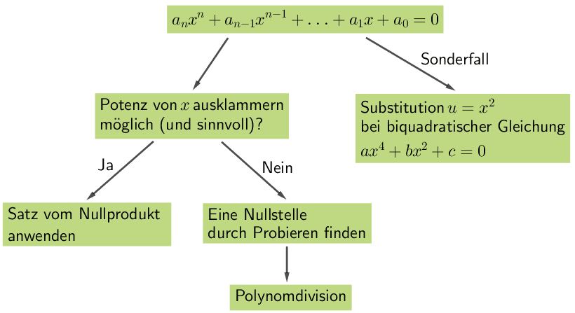
\[\begin{align*}\textcolor{#cc071e}{a}x^2 + \textcolor{#0087c1}{b}x &= 0 &&| \; x\; \text{ausklammern (Produkt formulieren)} \\[0.8em] x \cdot (ax + b) &= 0 \\[0.8em] \Rightarrow \enspace x = 0 \vee ax + b &= 0 \end{align*}\]
\[\begin{align*}\textcolor{#cc071e}{a}x^2 + \textcolor{#e9b509}{c} &= 0 &&| -c \enspace (c \neq 0) \\[0.8em] ax^2 &= -c &&| : a \\[0.8em] x^2 &= -\frac{c}{a} &&| \; \sqrt{\quad} \\[0.8em] x_{1,2} &= \pm \sqrt{-\frac{c}{a}} \end{align*}\]
Zwei Lösungen, falls \(-\dfrac{c}{a} > 0\), keine Lösung, falls \(-\dfrac{c}{a} < 0\)
Vorgehensweise für die Bestimmung der Nullstelle(n) einer ganzrationalen Funktion ab Grad 3:
vgl. Abiturskript - 1.1.3 Ganzrationale Funktion, Nullstellen
Nullstellen einer gebrochenrationalen Funktion \(f(x) = \dfrac{\textcolor{#0087c1}{z(x)}}{n(x)}\) sind alle Nullstellen des Zählerpolynoms \(\textcolor{#0087c1}{z(x)}\), die nicht zugleich Nullstellen des Nennerpolynoms \(\boldsymbol{n(x)}\) sind.
Ist \(x_0\) eine Nullstelle des Zählerpolynoms \(\boldsymbol{z(x)}\) und zugleich eine vollständig kürzbare Nullstelle des Nennerpolynoms \(\boldsymbol{n(x)}\), so besitzt die gebrochenrationale Funktion \(f\) an der Stelle \(x_0\) eine hebbare Definitionslücke.
(vgl. Abiturskript - 1.2.1 Gebrochenrationale Funktion, Nullstellen und Polstellen)
Eine Wurzelfunktion \(f(x) = \sqrt{\textcolor{#cc071e}{g(x)}}\) nimmt genau dann den Wert null an, wenn der Radikand (Term unter der Wurzel) null ist.
\[\sin{x} = 0 \enspace \Rightarrow \enspace x = k \cdot \pi \; (k \in \mathbb Z)\]
\[\cos{x} = 0 \enspace \Rightarrow \enspace x = \dfrac{\pi}{2} + k \cdot \pi \; (k \in \mathbb Z)\]
Die natürliche Logarithmusfunktion \(x \mapsto \ln{x}\) besitzt die einzige Nullstelle \(\boldsymbol{x = 1}\).
\[\ln{\left( \textcolor{#0087c1}{f(x)} \right)} = 0 \enspace \Rightarrow \enspace \textcolor{#0087c1}{f(x) = 1}\]
Die natürliche Exponentialfunktion \(x \mapsto e^x\) sowie jede verkettete Funktion \(x \mapsto e^{f(x)}\) besitzt keine Nullstelle!
\[\begin{align*} \textcolor{#e9b509}{\overline{OX}'(\lambda)} &\textcolor{#e9b509}{=} \textcolor{#e9b509}{0} \\[0.8em] \frac{10\lambda + 20}{2\sqrt{5\lambda^{2} + 20\lambda + 265}} &= 0 \\[0.8em] \Rightarrow \enspace 10\lambda + 20 &= 0 &&| - 20 \\[0.8em] 10\lambda &= -20 &&| : 10 \\[0.8em] \lambda &= \textcolor{#89ba17}{-2}\end{align*}\]
Durch Einsetzen des Parameterwerts \(\lambda = \textcolor{#89ba17}{-2}\) in die Gleichung der Gerade \(g\) erhält man den Ortsvektor \(\textcolor{#0087c1}{\overrightarrow{F}}\).
\[F \in g \colon \textcolor{#0087c1}{\overrightarrow{F}} = \begin{pmatrix} -12 + \textcolor{#89ba17}{(-2)}\\ 11 + 2 \cdot \textcolor{#89ba17}{(-2)} \\ 0 \end{pmatrix} = \textcolor{#0087c1}{\begin{pmatrix} -14 \\ 7 \\ 0 \end{pmatrix}}\]
Länge der kürzestmögliche Strecke von der Uferlinie zur Boje berechnen:
Betrag eines Vektors
\[ \vert \overrightarrow{a} \vert = \sqrt{\overrightarrow{a} \circ \overrightarrow{a}} = \sqrt{{a_1}^2 + {a_2}^2 + {a_3}^2}\]
(vgl. Merkhilfe)
\[\begin{align*}d(O;g) &= \vert \textcolor{#0087c1}{\overrightarrow{F}} \vert = \left| \textcolor{#0087c1}{\begin{pmatrix} -14 \\ 7 \\ 0 \end{pmatrix}} \right| = \sqrt{(-14)^2 + 7^2 + 0^2} \\[0.8em] &= \sqrt{245} = 7\sqrt{5} \approx 15{,}7\end{align*}\]
Der Fotograf schwimmt eine Strecke von knapp 16 m.