Sei \(F\) der Lotfußpunkt des Lotes des Punktes \(P\) auf die Gerade \(g\), so lässt sich der Abstand \(d(P;g)\) des Punktes \(P\) von der Geraden \(g\) bestimmen, indem man die Länge des Verbindungsvektors \(\overrightarrow{PF}\) berechnet.
\[d(P;g) = d(P;F) = \vert \overrightarrow{PF} \vert\]
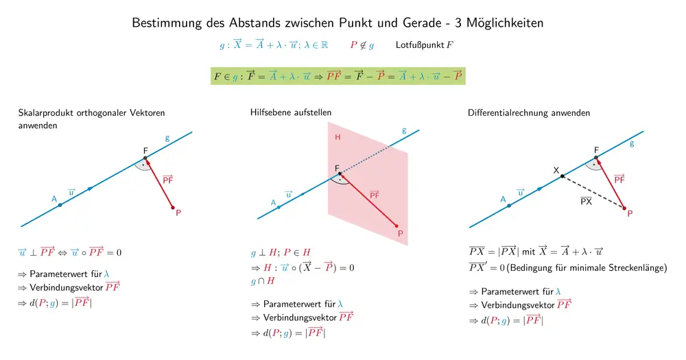
Es gibt mehrere Möglichkeiten, den Verbindungsvektor \(\overrightarrow{PF}\) zu ermitteln.
![]() Bestimmung des Abstands zwischen Punkt und Gerade - 3 Möglichkeiten
Bestimmung des Abstands zwischen Punkt und Gerade - 3 Möglichkeiten
1. Möglichkeit: Skalarprodukt orthogonaler (senkrechter) Vektoren anwenden

Der Richtungsvektor \(\overrightarrow{u}\) der Geraden \(g\) und der Verbindungsvektor \(\overrightarrow{PF}\) stehen senkrecht zueinander. Folglich ist das Skalarprodukt beider Vektoren gleich Null (vgl. Abiturskript - 2.1.3 Skalarprodukt von Vektoren, Anwendungen des Skalarprodukts).
\[\overrightarrow{u} \perp \overrightarrow{PF} \quad \Longleftrightarrow \quad \overrightarrow{u} \circ \overrightarrow{PF} = 0\]
Der Verbindungsvektor \(\overrightarrow{PF}\) lässt sich in Abhängigkeit des Parameters \(\lambda\) der Gleichung der Geraden \(g\) beschreiben.
\[g \colon \overrightarrow{X} = \overrightarrow{A} + \lambda \cdot \overrightarrow{u}; \; \lambda \in \mathbb R\]
\[F \in g \colon \overrightarrow{F} = \overrightarrow{A} + \lambda \cdot \overrightarrow{u}; \; \lambda \in \mathbb R\]
\[\overrightarrow{PF} = \overrightarrow{F} - \overrightarrow{P} = \overrightarrow{A} + \lambda \cdot \overrightarrow{u} - \overrightarrow{P}\]
Wendet man das Skalarprodukt der beiden orthogonalen Vektoren \(\overrightarrow{u}\) und \(\overrightarrow{PF}\) an, liefert dies genau den Wert des Parameters \(\lambda\), der den Verbindungsvektor \(\overrightarrow{PF}\) festlegt.
\[\begin{align*}\overrightarrow{u} \circ \overrightarrow{PF} &= 0 \\[0.8em] \overrightarrow{u} \circ (\overrightarrow{A} + \lambda \cdot \overrightarrow{u} - \overrightarrow{P}) &= 0 \end{align*}\]
\(\Longrightarrow \quad\)Parameterwert für \(\lambda\)
\(\Longrightarrow \quad \)Verbindungsvektor \(\overrightarrow{PF}\)
\[\Longrightarrow \quad d(P;g) = \vert \overrightarrow{PF} \vert\]
Beispiel:
Gegeben sei die Gerade \(g \colon \overrightarrow{X} = \begin{pmatrix} 6 \\ 3 \\ 2 \end{pmatrix} + \lambda \cdot \begin{pmatrix} -3 \\ 0 \\ 1 \end{pmatrix}; \; \lambda \in \mathbb R\) sowie der Punkt \(P(-4|8|2)\).
Bestimmen Sie den Abstand des Punktes \(P\) von der Geraden \(g\).
\[g \colon \overrightarrow{X} = \begin{pmatrix} 6 \\ 3 \\ 2 \end{pmatrix} + \lambda \cdot \begin{pmatrix} -3 \\ 0 \\ 1 \end{pmatrix}; \; \lambda \in \mathbb R\]
\[P(-4|8|2)\]
Verbindungsvektor \(\overrightarrow{PF}\) in Abhängigkeit des Parameters \(\lambda\) der Gleichung der Geraden \(g\) beschreiben:
\[F \in g \colon \overrightarrow{F} = \begin{pmatrix} 6 \\ 3 \\ 2 \end{pmatrix} + \lambda \cdot \begin{pmatrix} -3 \\ 0 \\ 1 \end{pmatrix} = \begin{pmatrix} 6 - 3\lambda \\ 3 \\ 2 + \lambda \end{pmatrix}\]
\[\overrightarrow{PF} = \overrightarrow{F} - \overrightarrow{P} = \begin{pmatrix} 6 - 3\lambda \\ 3 \\ 2 + \lambda \end{pmatrix} - \begin{pmatrix} -4 \\ 8 \\ 2 \end{pmatrix} = \begin{pmatrix} 10 - 3\lambda \\ -5 \\ \lambda \end{pmatrix}\]
Skalarprodukt der ortogonalen Vektoren \(\overrightarrow{u}\) und \(\overrightarrow{PF}\) anwenden (vgl. Abiturskript - 2.1.3 Skalarprodukt von Vektoren, Anwendungen des Skalarprodukts):
\[\begin{align*}\overrightarrow{u} \circ \overrightarrow{PF} &= 0 \\[0.8em] \begin{pmatrix} -3 \\ 0 \\ 1 \end{pmatrix} \circ \begin{pmatrix} 10 - 3\lambda \\ -5 \\ \lambda \end{pmatrix} &= 0 \\[0.8em] (-3) \cdot (10 - 3\lambda) + 0 \cdot (-5) + 1 \cdot \lambda &= 0 \\[0.8em] -30 + 10\lambda &= 0 & &| + 30 \\[0.8em] 10\lambda &= 30 & &| : 10 \\[0.8em] \lambda &= 3 \end{align*}\]
Verbindungsvektor \(\overrightarrow{PF}\) berechnen:
\[\overrightarrow{PF} = \begin{pmatrix} 10 - 3\lambda \\ -5 \\ \lambda \end{pmatrix} = \begin{pmatrix} 10 - 3 \cdot 3 \\ -5 \\ 3 \end{pmatrix} = \begin{pmatrix} 1 \\ -5 \\ 3 \end{pmatrix}\]
Abstand des Punktes \(P\) von der Geraden \(g\) berechnen:
\[d(P;g) = \vert \overrightarrow{PF} \vert = \left| \begin{pmatrix} 1 \\ -5 \\ 3 \end{pmatrix} \right| = \sqrt{1^{2} + (-5)^{2} + 3^{2}} = \sqrt{35} \approx 5{,}92\]
2. Möglichkeit: Hilfsebene aufstellen

Die Hilfsebene \(H\) mit den Eigenschaften \(P \in H\) und \(g \perp H\) schneidet die Gerade \(g\) im Lotfußpunkt \(F\) des Lotes des Punktes \(P\) auf die Gerade \(g\).
Um den Verbindungsvektor \(\overrightarrow{PF}\) zu bestimmen, stellt man eine Hilfsebene \(H\) auf, welche den Punkt \(P\) enthält und senkrecht zur Geraden \(g\) liegt. Als Normalenvektor für die Gleichung der Hilfsebene \(H\) in Normalenform dient der Richtungsvektor \(\overrightarrow{u}\) der Geradengleichung von \(g\).
\[P \in H\]
\[g \perp H \quad \Longrightarrow \quad \overrightarrow{n}_{H} = \overrightarrow{u}\]
\[H \colon \overrightarrow{u} \circ (\overrightarrow{X} - \overrightarrow{P}) = 0\]
Der Verbindungsvektor \(\overrightarrow{PF}\) lässt sich in Abhängigkeit des Parameters \(\lambda\) der Gleichung der Geraden \(g\) beschreiben.
\[g \colon \overrightarrow{X} = \overrightarrow{A} + \lambda \cdot \overrightarrow{u}\,; \; \lambda \in \mathbb R\]
\[F \in g \colon \overrightarrow{F} = \overrightarrow{A} + \lambda \cdot \overrightarrow{u}\,; \; \lambda \in \mathbb R\]
\[\overrightarrow{PF} = \overrightarrow{F} - \overrightarrow{P} = \overrightarrow{A} + \lambda \cdot \overrightarrow{u} - \overrightarrow{P}\]
Schneidet man die Geraden \(g\) mit der Hilfsebene \(H\), erhält man genau den Wert des Parameters \(\lambda\), der den Verbindungsvektor \(\overrightarrow{PF}\) festlegt (vgl. Abiturskript - 2.3.2 Lagebeziehung von Gerade und Ebene, Bestimmung des Schnittpunkts).
\[g \cap H \colon \overrightarrow{u} \circ (\overrightarrow{A} + \lambda \cdot \overrightarrow{u} - \overrightarrow{P}) = 0\]
\(\Longrightarrow \quad\)Parameterwert für \(\lambda\)
\(\Longrightarrow \quad \)Verbindungsvektor \(\overrightarrow{PF}\)
\[\Longrightarrow \quad d(P;g) = \vert \overrightarrow{PF} \vert\]
Beispiel (vgl. 1. Möglichkeit):
Gegeben sei die Gerade \(g \colon \overrightarrow{X} = \begin{pmatrix} 6 \\ 3 \\ 2 \end{pmatrix} + \lambda \cdot \begin{pmatrix} -3 \\ 0 \\ 1 \end{pmatrix}; \; \lambda \in \mathbb R\) sowie der Punkt \(P(-4|8|2)\).
Bestimmen Sie den Abstand des Punktes \(P\) von der Geraden \(g\).
\[g \colon \overrightarrow{X} = \begin{pmatrix} 6 \\ 3 \\ 2 \end{pmatrix} + \lambda \cdot \begin{pmatrix} -3 \\ 0 \\ 1 \end{pmatrix}; \; \lambda \in \mathbb R\]
\[P(-4|8|2)\]
Gleichung der Hilfsebene \(H\) aufstellen:
\(P \in H\,, \; g \perp H\)
\[H \colon \overrightarrow{u} \circ (\overrightarrow{X} - \overrightarrow{P}) = 0\]
\[H \colon \begin{pmatrix} -3 \\ 0 \\ 1 \end{pmatrix} \circ \left[ \overrightarrow{X} - \begin{pmatrix} -4 \\ 8 \\ 2 \end{pmatrix} \right] = 0\]
\[\begin{align*} \begin{pmatrix} -3 \\ 0 \\ 1 \end{pmatrix} \circ \left[ \overrightarrow{X} - \begin{pmatrix} -4 \\ 8 \\ 2 \end{pmatrix} \right] &= 0 \\[0.8em] (-3) \cdot (x_{1} + 4) + 0 \cdot (x_{2} - 8) + 1 \cdot (x_{3} - 2) &= 0 \\[0.8em] -3x_{1} - 12 + x_{3} - 2 &= 0 \\[0.8em] -3x_{1} + x_{3} - 14 &= 0 \end{align*}\]
\[H \colon -3x_{1} + x_{3} - 14 = 0\]
Verbindungsvektor \(\overrightarrow{PF}\) in Abhängigkeit des Parameters \(\lambda\) der Gleichung der Geraden \(g\) beschreiben:
\[F \in g \colon \overrightarrow{F} = \begin{pmatrix} 6 \\ 3 \\ 2 \end{pmatrix} + \lambda \cdot \begin{pmatrix} -3 \\ 0 \\ 1 \end{pmatrix} = \begin{pmatrix} 6 - 3\lambda \\ 3 \\ 2 + \lambda \end{pmatrix}\]
\[\overrightarrow{PF} = \overrightarrow{F} - \overrightarrow{P} = \begin{pmatrix} 6 - 3\lambda \\ 3 \\ 2 + \lambda \end{pmatrix} - \begin{pmatrix} -4 \\ 8 \\ 2 \end{pmatrix} = \begin{pmatrix} 10 - 3\lambda \\ -5 \\ \lambda \end{pmatrix}\]
Gerade \(g\) mit der Hilfsebene \(H\) schneiden (vgl. Abiturskript - 2.3.2 Lagebeziehung von Gerade und Ebene, Bestimmung des Schnittpunkts):
\[g \colon \overrightarrow{X} = \begin{pmatrix} 6 \\ 3 \\ 2 \end{pmatrix} + \lambda \cdot \begin{pmatrix} -3 \\ 0 \\ 1 \end{pmatrix}; \; \lambda \in \mathbb R\]
\[H \colon -3x_{1} + x_{3} - 14 = 0\]
\[\begin{align*} g \cap H \colon (-3) \cdot (6 - 3\lambda) + 2 + \lambda - 14 &= 0 \\[0.8em] -18 + 9\lambda + 2 + \lambda - 14 &= 0 \\[0.8em] -30 + 10\lambda &= 0 & &| + 30 \\[0.8em] 10\lambda &= 30 & &| : 10 \\[0.8em] \lambda &= 3 \end{align*}\]
Verbindungsvektor \(\overrightarrow{PF}\) berechnen:
\[\overrightarrow{PF} = \begin{pmatrix} 10 - 3\lambda \\ -5 \\ \lambda \end{pmatrix} = \begin{pmatrix} 10 - 3 \cdot 3 \\ -5 \\ 3 \end{pmatrix} = \begin{pmatrix} 1 \\ -5 \\ 3 \end{pmatrix}\]
Abstand des Punktes \(P\) von der Geraden \(g\) berechnen:
\[d(P;g) = \vert \overrightarrow{PF} \vert = \left| \begin{pmatrix} 1 \\ -5 \\ 3 \end{pmatrix} \right| = \sqrt{1^{2} + (-5)^{2} + 3^{2}} = \sqrt{35} \approx 5{,}92\]
3. Möglichkeit: Differentialrechnung anwenden (Extremwertaufgabe)
![Strecke [PX] zwischen dem Punkt P und einem beliebigen Punkt X ∈ g](/images/stories/abi_check/geometrie/Abstand_Punkt_Gerade4.png "Strecke [PX] zwischen dem Punkt P und einem beliebigen Punkt X ∈ g")
Strecke \([PX]\) zwischen Punkt \(P\) und einem beliebigen Punkt \(X \in g\)
Es sei \(F\) der Lotfußpunkt des Lotes des Punktes \(P\) auf die Gerade \(g\).
Die Länge der Strecke \([PX]\) zwischen dem Punkt \(P\) und einem beliebigen Punkt \(X \in g\) ist gleich dem Betrag des Verbindungsvektors \(\overrightarrow{PX}\).
\[\overline{PX} = \vert \overrightarrow{PX} \vert\]
Der Verbindungsvektor \(\overrightarrow{PX}\) lässt sich in Abhängigkeit des Parameters \(\lambda\) der Gleichung der Geraden \(g\) beschreiben.
\[g \colon \overrightarrow{X} = \overrightarrow{A} + \lambda \cdot \overrightarrow{u}\,; \; \lambda \in \mathbb R\]
\[\overrightarrow{PX} = \overrightarrow{X} - \overrightarrow{P} = \overrightarrow{A} + \lambda \cdot \overrightarrow{u} - \overrightarrow{P}\]
Für \(X = F\) ist die Länge der Strecke \([PX]\) minimal. Folglich muss die erste Ableitung \(\overline{PX}'\) gleich Null sein (vgl. Abiturskript - 1.5.3 Monotonieverhalten, Extrem- und Terrassenpunkte und Abiturskript - 1.5.7 Extremwertaufgaben). Der Nachweis der Art des Extremwerts kann entfallen, denn für \(X \neq F\) nimmt die Länge der Strecke \([PX]\) einen beliebig großen Wert an. Somit existiert keine maximale Länge der Strecke \([PX]\).
Die Extremstelle \(\lambda_{min}\) liefert genau den Wert des Parameters \(\lambda\), der den Verbindungsvektor \(\overrightarrow{PF}\) festlegt.
\[\overline{PX}' \overset{!}{=} 0\]
\(\Longrightarrow \quad\)Parameterwert für \(\lambda\)
\(\Longrightarrow \quad \)Verbindungsvektor \(\overrightarrow{PF}\)
\[\Longrightarrow \quad d(P;g) = \vert \overrightarrow{PF} \vert\]
Beispiel (vgl. 1. und 2. Möglichkeit):
Gegeben sei die Gerade \(g \colon \overrightarrow{X} = \begin{pmatrix} 6 \\ 3 \\ 2 \end{pmatrix} + \lambda \cdot \begin{pmatrix} -3 \\ 0 \\ 1 \end{pmatrix}; \; \lambda \in \mathbb R\) sowie der Punkt \(P(-4|8|2)\).
Bestimmen Sie den Abstand des Punktes \(P\) von der Geraden \(g\).
\[g \colon \overrightarrow{X} = \begin{pmatrix} 6 \\ 3 \\ 2 \end{pmatrix} + \lambda \cdot \begin{pmatrix} -3 \\ 0 \\ 1 \end{pmatrix}; \; \lambda \in \mathbb R\]
\[P(-4|8|2)\]
Verbindungsvektor \(\overrightarrow{PX}\) in Abhängigkeit des Parameters \(\lambda\) der Gleichung der Geraden \(g\) beschreiben:
\[g \colon \overrightarrow{X} = \begin{pmatrix} 6 \\ 3 \\ 2 \end{pmatrix} + \lambda \cdot \begin{pmatrix} -3 \\ 0 \\ 1 \end{pmatrix} = \begin{pmatrix} 6 - 3\lambda \\ 3 \\ 2 + \lambda \end{pmatrix}\]
\[\overrightarrow{PX} = \overrightarrow{X} - \overrightarrow{P} = \begin{pmatrix} 6 - 3\lambda \\ 3 \\ 2 + \lambda \end{pmatrix} - \begin{pmatrix} -4 \\ 8 \\ 2 \end{pmatrix} = \begin{pmatrix} 10 - 3\lambda \\ -5 \\ \lambda \end{pmatrix}\]
Länge der Strecke \([PX]\) in Abhängigkeit des Parameters \(\lambda\) formulieren:
\[\begin{align*} \overline{PX} &= \vert \overrightarrow{PX} \vert \\[0.8em] &= \left| \begin{pmatrix} 10 - 3\lambda \\ -5 \\ \lambda \end{pmatrix} \right| \\[0.8em] &= \sqrt{(10 - 3\lambda)^{2} + (-5)^{2} + \lambda^{2}} \\[0.8em] &= \sqrt{100 - 60\lambda + 9\lambda^{2} + 25 + \lambda^{2}} \\[0.8em] &= \sqrt{10\lambda^{2} - 60\lambda + 125} \end{align*}\]
Notwendige Bedingung \(\overline{PX}' = 0\) für minimale Länge der Strecke \([PX]\) (vgl. Abiturskript - 1.5.2 Ableitungsregeln):
\[\begin{align*} \overline{PX}' &= 0 \\[0.8em] \left( \sqrt{10\lambda^{2} - 60\lambda + 125} \right)' &= 0 \\[0.8em] \frac{20\lambda - 60}{2 \cdot \sqrt{10\lambda^{2} - 60\lambda + 125}} &= 0 \end{align*}\]
\[\begin{align*}\Longrightarrow \quad 20\lambda - 60 &= 0 & &| + 60 \\[0.8em] 20\lambda &= 60 & &| : 20 \\[0.8em] \lambda &= 3\end{align*}\]
Verbindungsvektor \(\overrightarrow{PF}\) berechnen:
\[\overrightarrow{PF} = \begin{pmatrix} 10 - 3\lambda \\ -5 \\ \lambda \end{pmatrix} = \begin{pmatrix} 10 - 3 \cdot 3 \\ -5 \\ 3 \end{pmatrix} = \begin{pmatrix} 1 \\ -5 \\ 3 \end{pmatrix}\]
Abstand des Punktes \(P\) von der Geraden \(g\) berechnen:
\[d(P;g) = \vert \overrightarrow{PF} \vert = \left| \begin{pmatrix} 1 \\ -5 \\ 3 \end{pmatrix} \right| = \sqrt{1^{2} + (-5)^{2} + 3^{2}} = \sqrt{35} \approx 5{,}92\]
Beispielaufgabe
Im Folgenden wird ein ebenes Gelände betrachtet, das modellhaft durch die \(x_{1}x_{2}\)-Ebene repräsentiert wird.
Ein Flugzeug startet im Punkt \(P(-10|-20|0)\) entlang der Geraden \(g \colon \overrightarrow{X} = \overrightarrow{P} + \lambda \cdot \begin{pmatrix} 5 \\ 5 \\ 1 \end{pmatrix}; \; \lambda \in \mathbb R\). Im Punkt \(R(80|94|0)\) befindet sich eine Radarstation mit einer Reichweite von 50 km. Es gilt: 1 LE (Längeneinheit) entspricht 1 km.
Begründen Sie durch Rechnung, dass das Flugzeug von der Radarstation erfasst wird.
\[P(-10|-20|0)\]
\[g \colon \overrightarrow{X} = \overrightarrow{P} + \lambda \cdot \begin{pmatrix} 5 \\ 5 \\ 1 \end{pmatrix}; \; \lambda \in \mathbb R\]
\[R(80|94|0)\]
Das Flugzeug wird von der Radarstation erfasst, wenn der Abstand \(d(R;g)\)des Punktes \(R\) von der Geraden \(g\) kleiner ist als die Reichweite der Radarstation.
1. Möglichkeit: Skalarprodukt orthogonaler (senkrechter) Vektoren anwenden

Es sei \(F\) der Lotfußpunkt des Lotes des Punktes \(R\) auf die Gerade \(g\).
\[g \colon \overrightarrow{X} = \begin{pmatrix} -10 \\ -20 \\ 0 \end{pmatrix} + \lambda \cdot \begin{pmatrix} 5 \\ 5 \\ 1 \end{pmatrix}; \; \lambda \in \mathbb R\]
\[R(80|94|0)\]
Verbindungsvektor \(\overrightarrow{RF}\) in Abhängigkeit des Parameters \(\lambda\) der Gleichung der Geraden \(g\) beschreiben:
\[F \in g \colon \overrightarrow{F} = \begin{pmatrix} -10 \\ -20 \\ 0 \end{pmatrix} + \lambda \cdot \begin{pmatrix} 5 \\ 5 \\ 1 \end{pmatrix} = \begin{pmatrix} -10 + 5\lambda \\ -20 + 5\lambda \\ \lambda \end{pmatrix}\]
\[\overrightarrow{RF} = \overrightarrow{F} - \overrightarrow{R} = \begin{pmatrix} -10 + 5\lambda \\ -20 + 5\lambda \\ \lambda \end{pmatrix} - \begin{pmatrix} 80 \\ 94 \\ 0 \end{pmatrix} = \begin{pmatrix} -90 + 5\lambda \\ -114 + 5\lambda \\ \lambda \end{pmatrix}\]
Skalarprodukt der ortogonalen Vektoren \(\overrightarrow{u}\) und \(\overrightarrow{RF}\) anwenden (vgl. Abiturskript - 2.1.3 Skalarprodukt von Vektoren, Anwendungen des Skalarprodukts):
\[\begin{align*}\overrightarrow{u} \circ \overrightarrow{RF} &= 0 \\[0.8em] \begin{pmatrix} 5 \\ 5 \\ 1 \end{pmatrix} \circ \begin{pmatrix} -90 + 5\lambda \\ -114 + 5\lambda \\ \lambda \end{pmatrix} &= 0 \\[0.8em] 5 \cdot (-90 + 5\lambda) + 5 \cdot (-114 + 5\lambda) + 1 \cdot \lambda &= 0 \\[0.8em] -450 + 25\lambda - 570 + 25\lambda + \lambda &= 0 \\[0.8em] -1020 + 51\lambda &= 0 & &| + 1020 \\[0.8em] 51\lambda &= 1020 & &| : 51 \\[0.8em] \lambda &= 20 \end{align*}\]
Verbindungsvektor \(\overrightarrow{RF}\) berechnen:
\[\overrightarrow{RF} = \begin{pmatrix} -90 + 5\lambda \\ -114 + 5\lambda \\ \lambda \end{pmatrix} = \begin{pmatrix} -90 + 5 \cdot 20 \\ -114 + 5 \cdot 20 \\ 20 \end{pmatrix} = \begin{pmatrix} 10 \\ -14 \\ 20 \end{pmatrix}\]
Abstand des Punktes \(R\) von der Geraden \(g\) berechnen:
\[d(R;g) = \vert \overrightarrow{RF} \vert = \left| \begin{pmatrix} 10 \\ -14 \\ 20 \end{pmatrix} \right| = \sqrt{10^{2} + (-14)^{2} + 20^{2}} = \sqrt{696} \approx 26{,}4\]
Mit ca. 26,4 km ist die kürzeste Entfernung des Flugzeugs von der Radarstation deutlich kleiner als die Reichweite der Radarstation (50 km). Folglich wird das Flugzeug von der Radarstation erfasst.
2. Möglichkeit: Hilfsebene aufstellen

Es sei \(F\) der Lotfußpunkt des Lotes des Punktes \(R\) auf die Gerade \(g\).
\[g \colon \overrightarrow{X} = \begin{pmatrix} -10 \\ -20 \\ 0 \end{pmatrix} + \lambda \cdot \begin{pmatrix} 5 \\ 5 \\ 1 \end{pmatrix}; \; \lambda \in \mathbb R\]
\[R(80|94|0)\]
Gleichung der Hilfsebene \(H\) aufstellen:
\(R \in H\,, \; g \perp H\)
\[H \colon \overrightarrow{u} \circ (\overrightarrow{X} - \overrightarrow{R}) = 0\]
\[H \colon \begin{pmatrix} 5 \\ 5 \\ 1 \end{pmatrix} \circ \left[ \overrightarrow{X} - \begin{pmatrix} 80 \\ 94 \\ 0 \end{pmatrix} \right] = 0\]
\[\begin{align*} \begin{pmatrix} 5 \\ 5 \\ 1 \end{pmatrix} \circ \left[ \overrightarrow{X} - \begin{pmatrix} 80 \\ 94 \\ 0 \end{pmatrix} \right] &= 0 \\[0.8em] 5 \cdot (x_{1} - 80) + 5 \cdot (x_{2} - 94) + 1 \cdot x_{3} &= 0 \\[0.8em] 5x_{1} - 400 + +5x_{2} - 470 + x_{3} &= 0 \\[0.8em] 5x_{1} + 5x_{2} + x_{3} - 870 &= 0 \end{align*}\]
\[H \colon 5x_{1} + 5x_{2} + x_{3} - 870 = 0\]
Verbindungsvektor \(\overrightarrow{RF}\) in Abhängigkeit des Parameters \(\lambda\) der Gleichung der Geraden \(g\) beschreiben:
\[F \in g \colon \overrightarrow{F} = \begin{pmatrix} -10 \\ -20 \\ 0 \end{pmatrix} + \lambda \cdot \begin{pmatrix} 5 \\ 5 \\ 1 \end{pmatrix} = \begin{pmatrix} -10 + 5\lambda \\ -20 + 5\lambda \\ \lambda \end{pmatrix}\]
\[\overrightarrow{RF} = \overrightarrow{F} - \overrightarrow{R} = \begin{pmatrix} -10 + 5\lambda \\ -20 + 5\lambda \\ \lambda \end{pmatrix} - \begin{pmatrix} 80 \\ 94 \\ 0 \end{pmatrix} = \begin{pmatrix} -90 + 5\lambda \\ -114 + 5\lambda \\ \lambda \end{pmatrix}\]
Geraden \(g\) mit der Hilfsebene \(H\) schneiden (vgl. Abiturskript - 2.3.2 Lagebeziehung von Gerade und Ebene, Bestimmung des Schnittpunkts):
\[g \colon \overrightarrow{X} = \begin{pmatrix} -10 \\ -20 \\ 0 \end{pmatrix} + \lambda \cdot \begin{pmatrix} 5 \\ 5 \\ 1 \end{pmatrix}; \; \lambda \in \mathbb R\]
\[H \colon 5x_{1} + 5x_{2} + x_{3} - 870 = 0\]
\[\begin{align*} g \cap H \colon 5 \cdot (-10 + 5\lambda) + 5 \cdot (-20 + 5\lambda) + \lambda - 870 &= 0 \\[0.8em] -50 + 25\lambda - 100 + 25\lambda + \lambda - 870 &= 0 \\[0.8em] -1020 + 51\lambda &= 0 & &| + 1020 \\[0.8em] 51\lambda &= 1020 & &| : 51 \\[0.8em] \lambda &= 20 \end{align*}\]
Verbindungsvektor \(\overrightarrow{RF}\) berechnen:
\[\overrightarrow{RF} = \begin{pmatrix} -90 + 5\lambda \\ -114 + 5\lambda \\ \lambda \end{pmatrix} = \begin{pmatrix} -90 + 5 \cdot 20 \\ -114 + 5 \cdot 20 \\ 20 \end{pmatrix} = \begin{pmatrix} 10 \\ -14 \\ 20 \end{pmatrix}\]
Abstand des Punktes \(R\) von der Geraden \(g\) berechnen:
\[d(R;g) = \vert \overrightarrow{RF} \vert = \left| \begin{pmatrix} 10 \\ -14 \\ 20 \end{pmatrix} \right| = \sqrt{10^{2} + (-14)^{2} + 20^{2}} = \sqrt{696} \approx 26{,}4\]
Mit ca. 26,4 km ist die kürzeste Entfernung des Flugzeugs von der Radarstation deutlich kleiner als die Reichweite der Radarstation (50 km). Folglich wird das Flugzeug von der Radarstation erfasst.
3. Möglichkeit: Differentialrechnung anwenden (Extremwertaufgabe)
![Strecke [RX] zwischen dem Punkt R und einem beliebigen Punkt X ∈ g](/images/stories/abi_check/geometrie/Abstand_Punkt_Gerade_Bsp3.png "Strecke [RX] zwischen dem Punkt R und einem beliebigen Punkt X ∈ g")
Es sei \(F\) der Lotfußpunkt des Lotes des Punktes \(R\) auf die Gerade \(g\).
\[g \colon \overrightarrow{X} = \begin{pmatrix} -10 \\ -20 \\ 0 \end{pmatrix} + \lambda \cdot \begin{pmatrix} 5 \\ 5 \\ 1 \end{pmatrix}; \; \lambda \in \mathbb R\]
\[R(80|94|0)\]
Verbindungsvektor \(\overrightarrow{RX}\) in Abhängigkeit des Parameters \(\lambda\) der Gleichung der Geraden \(g\) beschreiben:
\[g \colon \overrightarrow{X} = \begin{pmatrix} -10 \\ -20 \\ 0 \end{pmatrix} + \lambda \cdot \begin{pmatrix} 5 \\ 5 \\ 1 \end{pmatrix} = \begin{pmatrix} -10 + 5\lambda \\ -20 + 5\lambda \\ \lambda \end{pmatrix}\]
\[\overrightarrow{RX} = \overrightarrow{X} - \overrightarrow{R} = \begin{pmatrix} -10 + 5\lambda \\ -20 + 5\lambda \\ \lambda \end{pmatrix} - \begin{pmatrix} 80 \\ 94 \\ 0 \end{pmatrix} = \begin{pmatrix} -90 + 5\lambda \\ -114 + 5\lambda \\ \lambda \end{pmatrix}\]
Länge der Strecke \([RX]\) in Abhängigkeit des Parameters \(\lambda\) formulieren:
\[\begin{align*} \overline{RX} &= \vert \overrightarrow{RX} \vert \\[0.8em] &= \left| \begin{pmatrix} -90 + 5\lambda \\ -114 + 5\lambda \\ \lambda \end{pmatrix} \right| \\[0.8em] &= \sqrt{(-90 + 5\lambda)^{2} + (-114 + 5\lambda)^{2} + \lambda^{2}} \\[0.8em] &= \sqrt{8100 - 900\lambda + 25\lambda^{2} + 12996 - 1140\lambda + 25\lambda^{2} + \lambda^{2}} \\[0.8em] &= \sqrt{51\lambda^{2} - 2040\lambda + 21096} \end{align*}\]
Notwendige Bedingung \(\overline{RX}' = 0\) für minimale Länge der Strecke \([RX]\) (vgl. Abiturskript - 1.5.2 Ableitungsregeln):
\[\begin{align*} \overline{RX}' &= 0 \\[0.8em] \left( \sqrt{51\lambda^{2} - 2040\lambda + 21096} \right)' &= 0 \\[0.8em] \frac{102\lambda - 2040}{2 \cdot \sqrt{51\lambda^{2} - 2040\lambda + 21096}} &= 0 \end{align*}\]
\[\begin{align*}\Longrightarrow \quad 102\lambda - 2040 &= 0 & &| + 2040 \\[0.8em] 102\lambda &= 2040 & &| : 102 \\[0.8em] \lambda &= 20\end{align*}\]
Verbindungsvektor \(\overrightarrow{RF}\) berechnen:
\[\overrightarrow{RF} = \begin{pmatrix} -90 + 5\lambda \\ -114 + 5\lambda \\ \lambda \end{pmatrix} = \begin{pmatrix} -90 + 5 \cdot 20 \\ -114 + 5 \cdot 20 \\ 20 \end{pmatrix} = \begin{pmatrix} 10 \\ -14 \\ 20 \end{pmatrix}\]
Abstand des Punktes \(R\) von der Geraden \(g\) berechnen:
\[d(R;g) = \vert \overrightarrow{RF} \vert = \left| \begin{pmatrix} 10 \\ -14 \\ 20 \end{pmatrix} \right| = \sqrt{10^{2} + (-14)^{2} + 20^{2}} = \sqrt{696} \approx 26{,}4\]
Mit ca. 26,4 km ist die kürzeste Entfernung des Flugzeugs von der Radarstation deutlich kleiner als die Reichweite der Radarstation (50 km). Folglich wird das Flugzeug von der Radarstation erfasst.