Bestimmen Sie eine Gleichung der Ebene \(E\) in Koordinatenform und zeigen Sie, dass die Gerade \(g\) in \(E\) liegt.
(zur Kontrolle: \(E \colon 2x_1 - x_2 + 2x_3 + 35 = 0\))
(5 BE)
Lösung zu Teilaufgabe b
Gleichung der Ebene \(E\) in Koordinatenform
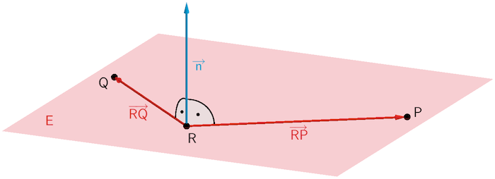
Die Punkte \(P\), \(Q\) und \(R\) liegen in der Ebene \(E\) (vgl. Angabe). Somit liefert beispielsweise das Vektorprodukt \(\textcolor{#cc071e}{\overrightarrow{RP} \times \overrightarrow{RQ}}\) der beiden linear unabhängigen Verbindungsvektoren \(\textcolor{#cc071e}{\overrightarrow{RP}}\) und \(\textcolor{#cc071e}{\overrightarrow{RQ}}\) einen Normalenvektor der Ebene \(E\). Als Aufpunkt wählt man einen der Punkte \(P\), \(Q\) oder \(R\). Damit lässt sich eine Gleichung der Ebene \(E\) in Koordinatenform (Normalenform in Koordinatendarstellung) bestimmen.
Lineare (Un)Abhängigkeit von zwei Vektoren
Zwei Vektoren \(\overrightarrow{a}\) und \(\overrightarrow{b}\) sind
linear abhängig, wenn
\(\overrightarrow{a} \parallel \overrightarrow{b}\) bzw. \(\overrightarrow{a} = k \cdot \overrightarrow{b}\) mit \(k \in \mathbb R\) gilt.
linear unabhängig, wenn
\(\overrightarrow{a} \nparallel \overrightarrow{b}\) bzw. \(\overrightarrow{a} \neq k \cdot \overrightarrow{b}\) mit \(k \in \mathbb R\) gilt.
Lineare (Un-)Abhängigkeit von drei Vektoren
Drei Vektoren \(\overrightarrow{a}\), \(\overrightarrow{b}\) und \(\overrightarrow{c}\) sind
linear abhängig, wenn
sie in einer Ebene liegen bzw. wenn beispielsweise
die lineare Vektorgleichung \(\overrightarrow{c} = r \cdot \overrightarrow{a} + s \cdot \overrightarrow{b}\) eine eindeutige Lösung hat.
linear unabhängig, wenn
sie den Raum \(\mathbb R^{3}\) aufspannen bzw. wenn beispielsweise
die lineare Vektorgleichung \(\overrightarrow{c} = r \cdot \overrightarrow{a} + s \cdot \overrightarrow{b}\) keine Lösung hat.
Der Ansatz kann mithilfe der Normalenform in Vektordarstellung oder in Koordinatendarstellung erfolgen.
Ebenengleichung in Normalenform (vgl. Merkhilfe)
Jede Ebene lässt sich durch eine Gleichung in Normalenform beschreiben. Ist \(A\) ein beliebiger Aufpunkt der Ebene \(E\) und \(\overrightarrow{n}_{E}\) ein Normalenvektor von \(E\), so erfüllt jeder Punkt \(X\) der Ebene \(E\) folgende Gleichungen:
Normalenform in Vektordarstellung
\[E \colon \overrightarrow{n}_{E} \circ (\overrightarrow{X} - \overrightarrow{A}) = 0\]

Normalenform in Koordinatendarstellung
\[E \colon n_{1}x_{1} + n_{2}x_{2} + n_{3}x_{3} + n_{0} = 0\]
mit \(n_{0} = -(\overrightarrow{n}_{E} \circ \overrightarrow{A}) = - \: n_{1}a_{1} - n_{2}a_{2} - n_{3}a_{3}\)
\(n_{1}\), \(n_{2}\) und \(n_{3}\): Koordinaten eines Normalenvektors \(\overrightarrow{n}_{E}\)
Die Verbindungsvektoren \(\textcolor{#cc071e}{\overrightarrow{RP}}\) und \(\textcolor{#cc071e}{\overrightarrow{RQ}}\) sollten aus Teilaufgabe a bekannt sein.
\(\textcolor{#cc071e}{\overrightarrow{RP}} = \textcolor{#cc071e}{\begin{pmatrix} 1 \\ -2 \\ -2 \end{pmatrix}}\); \(\textcolor{#cc071e}{\overrightarrow{RQ}} = \textcolor{#cc071e}{\begin{pmatrix} 2 \\ 2 \\ -1 \end{pmatrix}}\)
Normalenvektor \(\textcolor{#0087c1}{\overrightarrow{n}}\) der Ebene \(E\) ermitteln:
Vektorprodukt (Kreuzprodukt)
Das Vektorprodukt \(\overrightarrow{a} \times \overrightarrow{b}\) zweier Vektoren \(\overrightarrow{a}\) und \(\overrightarrow{b}\) erzeugt einen neuen Vektor \(\overrightarrow{c} = \overrightarrow{a} \times \overrightarrow{b}\) mit den Eigenschaften:
\(\overrightarrow{c}\) ist sowohl zu \(\overrightarrow{a}\) als auch zu \(\overrightarrow{b}\) senkrecht.
\[\overrightarrow{c} = \overrightarrow{a} \times \overrightarrow{b} \quad \Longrightarrow \quad \overrightarrow{c} \perp \overrightarrow{a}, \enspace \overrightarrow{c} \perp \overrightarrow{b}\]
Der Betrag des Vektorprodukts zweier Vektoren \(\overrightarrow{a}\) und \(\overrightarrow{b}\) ist gleich dem Produkt aus den Beträgen der Vektoren \(\overrightarrow{a}\) und \(\overrightarrow{b}\) und dem Sinus des von ihnen eingeschlossenen Winkels \(\varphi\).
\[\vert \overrightarrow{a} \times \overrightarrow{b} \vert = \vert \overrightarrow{a} \vert \cdot \vert \overrightarrow{b} \vert \cdot \sin{\varphi} \quad (0^{\circ} \leq \varphi \leq 180^{\circ})\]
Die Vektoren \(\overrightarrow{a}\), \(\overrightarrow{b}\) und \(\overrightarrow{c}\) bilden in dieser Reihenfolge ein Rechtssystem. Rechtehandregel: Weist \(\overrightarrow{a}\) in Richtung des Daumens und \(\overrightarrow{b}\) in Richtung des Zeigefingers, dann weist \(\overrightarrow{c} = \overrightarrow{a} \times \overrightarrow{b}\) in Richtung des Mittelfingers.
Berechnung eines Vektorprodukts im \(\boldsymbol{\mathbb R^{3}}\) (vgl. Merkhilfe)
\[\overrightarrow{a} \times \overrightarrow{b} = \begin {pmatrix} a_1 \\ a_2 \\ a_3 \end {pmatrix} \times \begin {pmatrix} b_1 \\ b_2 \\ b_3 \end {pmatrix} = \begin {pmatrix} a_2 \cdot b_3 - a_3 \cdot b_2 \\ a_3 \cdot b_1 - a_1 \cdot b_3 \\ a_1 \cdot b_2 - a_2 \cdot b_1 \end {pmatrix}\]
\[\begin{align*} \textcolor{#cc071e}{\overrightarrow{RP}} \times \textcolor{#cc071e}{\overrightarrow{RQ}} &= \textcolor{#cc071e}{\begin{pmatrix} 1 \\ -2 \\ -2 \end{pmatrix}} \times \textcolor{#cc071e}{\begin{pmatrix} 2 \\ 2 \\ -1 \end{pmatrix}} \\[0.8em] &= \begin{pmatrix} -2 & \cdot & (-1) & - & (-2) & \cdot & 2 \\ -2 & \cdot & 2 & - & 1 & \cdot & (-1) \\ 1 & \cdot & 2 & - & (-2) & \cdot & 2 \end{pmatrix} \\[0.8em] &= \begin{pmatrix} 6 \\ -3 \\ 6 \end{pmatrix} = 3 \cdot \begin{pmatrix} 2 \\ -1 \\ 2 \end{pmatrix} \end{align*}\]
Somit ist der Vektor \(\textcolor{#0087c1}{\overrightarrow{n} = \begin{pmatrix} 2 \\ -1 \\ 2 \end{pmatrix}}\) ein Normalenvektor der Ebene \(E\).
Gleichung der Ebene \(E\) in Koordinatenform bestimmen:
Der Punkt \(\textcolor{#e9b509}{R(4|5|-19)}\) dient beispielsweise als Aufpunkt.
1. Möglichkeit: Ansatz mit Normalenform in Vektordarstellung
Ebenengleichung in Normalenform (vgl. Merkhilfe)
Jede Ebene lässt sich durch eine Gleichung in Normalenform beschreiben. Ist \(A\) ein beliebiger Aufpunkt der Ebene \(E\) und \(\overrightarrow{n}_{E}\) ein Normalenvektor von \(E\), so erfüllt jeder Punkt \(X\) der Ebene \(E\) folgende Gleichungen:
Normalenform in Vektordarstellung
\[E \colon \overrightarrow{n}_{E} \circ (\overrightarrow{X} - \overrightarrow{A}) = 0\]
Normalenform in Koordinatendarstellung
\[E \colon n_{1}x_{1} + n_{2}x_{2} + n_{3}x_{3} + n_{0} = 0\]
mit \(n_{0} = -(\overrightarrow{n}_{E} \circ \overrightarrow{A}) = - \: n_{1}a_{1} - n_{2}a_{2} - n_{3}a_{3}\)
\(n_{1}\), \(n_{2}\) und \(n_{3}\): Koordinaten eines Normalenvektors \(\overrightarrow{n}_{E}\)
\[\begin{align*}E \colon &\,\textcolor{#0087c1}{\overrightarrow{n}} \circ (\overrightarrow{X} - \textcolor{#e9b509}{\overrightarrow{R})} = 0 \\[0.8em] E \colon &\textcolor{#0087c1}{\begin{pmatrix} 2 \\ -1 \\ 2 \end{pmatrix}} \circ \left[ \overrightarrow{X} - \textcolor{#e9b509}{\begin{pmatrix} 4 \\ 5 \\ -19 \end{pmatrix}} \right] = 0 \\[0.8em] &\,\textcolor{#0087c1}{2} \cdot (x_{1} - \textcolor{#e9b509}{4}) + \textcolor{#0087c1}{(-1)} \cdot (x_{2} - \textcolor{#e9b509}{5}) + \textcolor{#0087c1}{2} \cdot (x_{3} - \textcolor{#e9b509}{(-19)}) = 0 \\[0.8em] &\,2x_1 - 8 - x_2 + 5 + 2x_3 + 38 = 0 \\[0.8em] E \colon\, &2x_{1} - x_{2} + 2x_{3} + 35 = 0 \end{align*}\]
2. Möglichkeit: Ansatz mit Normalenform in Koordinatendarstellung
\(\textcolor{#0087c1}{\overrightarrow{n} = \begin{pmatrix} 2 \\ -1 \\ 2 \end{pmatrix}}\); \(\textcolor{#e9b509}{R(4|5|-19)}\)
Ebenengleichung in Normalenform (vgl. Merkhilfe)
Jede Ebene lässt sich durch eine Gleichung in Normalenform beschreiben. Ist \(A\) ein beliebiger Aufpunkt der Ebene \(E\) und \(\overrightarrow{n}_{E}\) ein Normalenvektor von \(E\), so erfüllt jeder Punkt \(X\) der Ebene \(E\) folgende Gleichungen:
Normalenform in Vektordarstellung
\[E \colon \overrightarrow{n}_{E} \circ (\overrightarrow{X} - \overrightarrow{A}) = 0\]
Normalenform in Koordinatendarstellung
\[E \colon n_{1}x_{1} + n_{2}x_{2} + n_{3}x_{3} + n_{0} = 0\]
mit \(n_{0} = -(\overrightarrow{n}_{E} \circ \overrightarrow{A}) = - \: n_{1}a_{1} - n_{2}a_{2} - n_{3}a_{3}\)
\(n_{1}\), \(n_{2}\) und \(n_{3}\): Koordinaten eines Normalenvektors \(\overrightarrow{n}_{E}\)
\[\begin{align*} &E \colon n_{1}x_{1} + n_{2}x_{2} + n_{3}x_{3} + n_{0} = 0 \\[0.8em] &E \colon \textcolor{#0087c1}{2} \cdot x_{1} + \textcolor{#0087c1}{(-1)} \cdot x_{2} + \textcolor{#0087c1}{2} \cdot x_{3} + n_{0} = 0\\[0.8em] &E\colon 2x_{1} - x_{2} + 2x_{3} + n_{0} = 0 \end{align*}\]
\[\begin{align*} \textcolor{#e9b509}{R} \in E \colon 2 \cdot \textcolor{#e9b509}{4} - \textcolor{#e9b509}{5} + 2 \cdot \textcolor{#e9b509}{(-19)} + n_{0} &= 0 \\[0.8em] 8 - 5 - 38 + n_{0} &= 0 \\[0.8em] -35 + n_0 &= 0 &&| + 35 \\[0.8em] n_{0} &= 35 \end{align*}\]
\[\Rightarrow \enspace E \colon 2x_{1} - x_{2} + 2x_{3} + 35 = 0\]
Nachweis, dass die Gerade \(g\) in \(E\) liegt
\[g \colon \overrightarrow{X} = \textcolor{#e9b509}{\begin{pmatrix} -12 \\ 11 \\ 0 \end{pmatrix}} + \lambda \cdot \textcolor{#89ba17}{\begin{pmatrix} 1 \\ 2 \\ 0 \end{pmatrix}}, \; \lambda \in \mathbb R\]
1. Möglichkeit: Richtungsvektor von \(g\) und Normalenvektor von \(E\) betrachten
Die Gerade \(g\) liegt in der Ebene \(E\), wenn der Richtungsvektor von \(g\) und der Normalenvektor von \(E\) zueinander senkrecht sind, wenn also das Skalarprodukt der beiden Vektoren gleich null ist, und außerdem der Aufpunkt von \(g\) die Gleichung der Ebene \(E\) erfüllt.
(vgl. ![]() Untersuchung der Lagebeziehung zwischen Gerade und Ebene, Abiturskript - 2.3.2 Lagebeziehung von Gerade und Ebene)
Untersuchung der Lagebeziehung zwischen Gerade und Ebene, Abiturskript - 2.3.2 Lagebeziehung von Gerade und Ebene)
Anwendung des Skalarprodukts:
Orthogonale (zueinander senkrechte) Vektoren (vgl. Merkhilfe)
\[\overrightarrow{a} \perp \overrightarrow{b} \; \Leftrightarrow \; \overrightarrow{a} \circ \overrightarrow{b} \quad (\overrightarrow{a} \neq \overrightarrow{0},\; \overrightarrow{b} \neq \overrightarrow{0})\]
\[g \colon \overrightarrow{X} = \begin{pmatrix} -12 \\ 11 \\ 0 \end{pmatrix} + \lambda \cdot \textcolor{#89ba17}{\begin{pmatrix} 1 \\ 2 \\ 0 \end{pmatrix}}, \; \lambda \in \mathbb R\]
Normalenvektor von \(E\): \(\textcolor{#0087c1}{\overrightarrow{n} = \begin{pmatrix} 2 \\ -1 \\ 2 \end{pmatrix}}\)
Skalarprodukt
Unter dem Skalarprodukt \(\overrightarrow{a} \circ \overrightarrow{b}\) zweier Vektoren \(\overrightarrow{a}\) und \(\overrightarrow{b}\) versteht man das Produkt aus den Beträgen der beiden Vektoren und dem Kosinus des von den Vektoren eingeschlossenen Winkels \(\varphi\).
\[\overrightarrow{a} \circ \overrightarrow{b} = \vert \overrightarrow{a} \vert \cdot \vert \overrightarrow{b} \vert \cdot \cos{\varphi} \quad (0^{\circ} \leq \varphi \leq 180^{\circ})\]
Berechnung eines Skalarprodukts im \(\boldsymbol{\mathbb R^{3}}\) (vgl. Merkhilfe)
\[\overrightarrow{a} \circ \overrightarrow{b} = \begin{pmatrix} a_{1} \\ a_{2} \\ a_{3} \end{pmatrix} \circ \begin{pmatrix} b_{1} \\ b_{2} \\ b_{3} \end{pmatrix} = a_{1}b_{1} + a_{2}b_{2} + a_{3}b_{3}\]
\[\textcolor{#89ba17}{\begin{pmatrix} 1 \\ 2 \\ 0 \end{pmatrix}} \circ \textcolor{#0087c1}{\begin{pmatrix} 2 \\ -1 \\ 2 \end{pmatrix}} = 1 \cdot 2 + 2 \cdot (-1) + 0 \cdot 2 = 0\]
Folglich sind der Richtungsvektor von \(g\) und der Normalenvektor von \(E\) zueinander senkrecht. Die Gerade \(g\) kann somit echt parallel zur Ebene \(E\) verlaufen oder in der Ebene \(E\) liegen.
Punktprobe, ob der Aufpunkt von \(g\) die Gleichung von \(E\) erfüllt:
\[g \colon \overrightarrow{X} = \textcolor{#e9b509}{\begin{pmatrix} -12 \\ 11 \\ 0 \end{pmatrix}} + \lambda \cdot \begin{pmatrix} 1 \\ 2 \\ 0 \end{pmatrix}, \; \lambda \in \mathbb R\]
\[E \colon 2x_{1} - x_{2} + 2x_{3} + 35 = 0\]
\[\begin{align*}2 \cdot \textcolor{#e9b509}{(-12)} - \textcolor{#e9b509}{11} + 2 \cdot \textcolor{#e9b509}{0} + 35 = 0 \\[0.8em] -24 - 11 + 35 &= 0 \\[0.8em] -35 + 35 &= 0 && (\text{w})\end{align*}\]
\[\Rightarrow \enspace \textcolor{#e9b509}{(-12|11|0)} \in E\]
Also liegt die Gerade \(g\) in der Ebene \(E\) (\(g \subset E\)).
2. Möglichkeit: Untersuchung der gemeinsamen Punkte von \(g\) und \(E\)
Hierfür werden die Koordinaten der Geradengleichung von \(g\) in die Gleichung der Ebene \(E\) eingesetzt. Die Gerade \(g\) liegt in der Ebene \(E\), wenn die Gleichung eine wahre Aussage liefert.
\[g \colon \overrightarrow{X} = \begin{pmatrix} -12 \\ 11 \\ 0 \end{pmatrix} + \lambda \cdot \begin{pmatrix} 1 \\ 2 \\ 0 \end{pmatrix} = \textcolor{#e9b509}{\begin{pmatrix} -12 + \lambda \\ 11 + 2\lambda \\ 0 \end{pmatrix}}, \; \lambda \in \mathbb R\]
\[E \colon 2x_{1} - x_{2} + 2x_{3} + 35 = 0\]
\[\begin{align*}g \cap E \colon 2 \cdot \textcolor{#e9b509}{(-12 + \lambda)}- \textcolor{#e9b509}{(11 + 2\lambda)} + 2 \cdot \textcolor{#e9b509}{0} + 35 &= 0 \\[0.8em] -24 + 2\lambda - 11 - 2\lambda + 35 &= 0 \\[0.8em] -35 + 35 &= 0 &&(\text{w}) \end{align*}\]
Also liegt die Gerade \(g\) in der Ebene \(E\) (\(g \subset E\)).