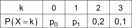
Bei einer Werbeaktion werden den Fruchtgummitüten Rubbellose beigelegt. Beim Freirubbeln werden auf dem Los bis zu drei Goldäpfel sichtbar. Die Zufallsgröße \(X\) beschreibt die Anzahl der Goldäpfel, die beim Freirubbeln sichtbar werden. Die Tabelle zeigt die Wahrscheinlichkeitsverteilung von \(X\).
Die Zufallsgröße \(X\) hat den Erwartungswert 1. Bestimmen Sie die Wahrscheinlichkeiten \(p_{0}\) und \(p_{1}\) und berechnen Sie die Varianz von \(X\).
(3 BE)
Lösung zu Teilaufgabe 4a
Bestimmung der Wahrscheinlichkeiten \(p_{0}\) und \(p_{1}\)
Da die Zufallsgröße \(X\) den Erwartungswert 1 hat (vgl. Angabe), folgt:
Ist \(X\) eine Zufallsgröße, deren mögliche Werte \(x_{1}, x_{2}, ..., x_{n}\) sind, dann gilt:
Erwartungswert \(\boldsymbol{\mu}\) einer Zufallsgröße \(\boldsymbol{X}\)
\[\begin{align*}\mu = E(X) &= \sum \limits_{i = 1}^{n} x_{i} \cdot P(X = x_i) \\[0.8em] &= x_{1} \cdot P(X = x_1) + x_{2} \cdot P(X = x_2) + \cdots + x_{n} \cdot P(X = x_n) \end{align*}\]
Der Erwartungswert \(\mu = E(X)\) gibt den Mittelwert einer Zufallsgröße \(X\) pro Versuch an, der bei sehr häufiger Durchführung eines Zufallsexperiments (auf lange Sicht) zu erwarten ist.
\[\begin{align*}E(X) &= 1\\[0.8em] 0 \cdot p_{0} + 1 \cdot p_{1} + 2 \cdot 0{,}2 + 3 \cdot 0{,}1 &= 1 \\[0.8em] p_{1} + 0{,}7 &= 1&&|-0{,}7\\[0.8em]\textcolor{#e9b509}{p_{1}}&= \textcolor{#e9b509}{0{,}3}\end{align*}\]
Außerdem ist die Summe der Wahrscheinlichkeiten \(P(X = k)\) gleich 1.
\[\begin{align*}\sum P(X = k) &= 1\\[0.8em]p_{0} + \textcolor{#e9b509}{p_{1}} + 0{,}2 + 0{,}1 &= 1 \\[0.8em] p_{0} + \textcolor{#e9b509}{0{,}3} + 0{,}2 + 0{,}1&= 1 \\[0.8em] p_{0} + 0{,}6 &= 1&&| -0{,}6\\[0.8em] p_{0} &= 0{,}4\end{align*}\]
Berechnung der Varianz von \(X\)
Wahrscheinlichkeitsverteilung der Zufallsgröße \(X\):
| \(k\) | \(\textcolor{#0087c1}{0}\) | \(\textcolor{#0087c1}{1}\) | \(\textcolor{#0087c1}{2}\) | \(\textcolor{#0087c1}{3}\) |
| \(P(X = k)\) | \(\textcolor{#e9b509}{0{,}4}\) | \(\textcolor{#e9b509}{0{,}3}\) | \(\textcolor{#e9b509}{0{,}2}\) | \(\textcolor{#e9b509}{0{,}1}\) |
\[\textcolor{#cc071e}{E(X)} = \textcolor{#cc071e}{1}\]
Ist \(X\) eine Zufallsgröße, deren mögliche Werte \(x_{1}, x_{2}, ..., x_{n}\) sind, dann gilt:
Varianz \(\boldsymbol{Var(X)}\) der Zufallsgröße \(\boldsymbol{X}\)
\[\begin{align*}Var(X) \enspace = \quad &\sum \limits_{i\;=\;1}^{n} (x_{i} - \mu)^{2} \cdot P(X = x_{i}) \\[0.8em] \enspace = \quad &(x_{1} - \mu)^{2} \cdot P(X = x_{1}) + (x_{2} - \mu)^{2} \cdot P(X = x_{2}) + \dots \\[0.8em] + \; &(x_n - \mu)^2 \cdot P(X = x_n)\end{align*}\]
Die Varianz \(\boldsymbol{Var(X)}\) einer Zufallsgröße \(X\) ist eine Maßzahl für die Streuung der Werte \(x_{i}\) der Zufallsgröße um den Erwartungswert \(\mu\).
\[\begin{align*}Var(X) &= (\textcolor{#0087c1}{0} - \textcolor{#cc071e}{1})^{2} \cdot \textcolor{#e9b509}{0{,}4}+(\textcolor{#0087c1}{1} - \textcolor{#cc071e}{1})^{2} \cdot \textcolor{#e9b509}{0{,}3}+(\textcolor{#0087c1}{2} - \textcolor{#cc071e}{1})^{2} \cdot \textcolor{#e9b509}{0{,}2}+(\textcolor{#0087c1}{3} - \textcolor{#cc071e}{1})^{2} \cdot \textcolor{#e9b509}{0{,}1} \\[0.8em] &= 0{,}4 + 0 + 0{,}2 + 0{,}4 \\[0.8em] &= 1 \end{align*}\]