Untersuchen Sie rechnerisch das Monotonieverhalten von \(f\). Ergänzen Sie in der Abbildung 1 die Koordinatenachsen und skalieren Sie diese passend.
(5 BE)
Lösung zu Teilaufgabe 1c
Rechnerische Untersuchung des Monotonieverhaltens von \(f\)
Gemäß dem Monotoniekriterium wird das Vorzeichen von \(f'\) betrachtet.
Anwendung der Differetialrechnung:
Monotoniekriterium
\(\textcolor{#cc071e}{f'(x) < 0}\) im Intervall \( I \; \Rightarrow \; G_{f}\) fällt streng monoton in \(I\)
\(\textcolor{#0087c1}{f'(x) > 0}\) im Intervall \( I \; \Rightarrow \; G_{f}\) steigt streng monoton in \(I\)
(vgl. Merkhilfe)
\[\begin{align*}f'(x) &= \textcolor{#89ba17}{(1 - x^2)} \cdot e^{-\frac{1}{2}x^2 + \frac{1}{2}} &&| \;\text{3. Bin. Formel anwenden} \\[0.8em] &= \textcolor{#89ba17}{(1 - x)(1 + x)} \cdot \textcolor{#e9b509}{\underbrace{e^{-\frac{1}{2}x^2 + \frac{1}{2}}}_{>\,0}} \end{align*}\]
Der Faktor \(\textcolor{#89ba17}{(1 - x^2)}\) mit den einfachen Nullstellen \(\textcolor{#89ba17}{x = -1}\) und \(\textcolor{#89ba17}{x = 1}\) bestimmt den Vorzeichenwechsel von \(\boldsymbol{f'}\).
Der quadratische Term \(\textcolor{#89ba17}{1 - x^2}\) lässt sich als nach unten geöffnete Normalparabel veranschaulichen, welche zwischen den Nullstellen oberhalb der \(\textcolor{#0087c1}{x}\)-Achse verläuft.
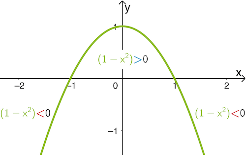
Somit folgt:
Da \(f'(x) \textcolor{#0087c1}{>} 0\) für \(\textcolor{#0087c1}{-1 < x < 1}\) gilt, ist \(f\) im Intervall \(\textcolor{#0087c1}{[-1;1]}\) streng monoton zunehmend.
Da \(f'(x) \textcolor{#cc071e}{<} 0\) für \(\textcolor{#cc071e}{x < -1}\) und \(\textcolor{#cc071e}{x > 1}\) gilt, ist \(f\) in den Intervallen \(\textcolor{#cc071e}{]-\infty;-1]}\) und \(\textcolor{#cc071e}{[1;+\infty[}\) streng monoton abnehmend.
Veranschaulichung mithilfe einer Monotonietabelle:
| \(x\) | \(]-\infty;-1]\) | \(-1\) | \([-1;1]\) | \(1\) | \([1;+\infty[\) |
| \(\textcolor{#89ba17}{(1 - x)}\) | \(\textcolor{#0087c1}{+}\) | \(\textcolor{#0087c1}{+}\) | \(0\) | \(\textcolor{#cc071e}{-}\) | |
| \(\textcolor{#89ba17}{(1 + x)}\) | \(\textcolor{#cc071e}{-}\) | \(0\) | \(\textcolor{#0087c1}{+}\) | \(\textcolor{#0087c1}{+}\) | |
| \(f'(x)\) | \(\textcolor{#cc071e}{-}\) | \(0\) | \(\textcolor{#0087c1}{+}\) | \(0\) | \(\textcolor{#cc071e}{-}\) |
| \(G_f\) | \(\textcolor{#cc071e}{\searrow}\) | \(TiP\) | \(\textcolor{#0087c1}{\nearrow}\) | \(HoP\) | \(\textcolor{#cc071e}{\searrow}\) |
Ergänzung und Skalierung der Koordinatenachsen in Abbildung 1
Aus dem Monotonieverhalten von \(f\) folgt, das \(G_f\) den Tiefpunkt \((-1|f(-1))\) und den Hochpunkt \((1|f(1))\) besitzt. Da \(G_f\) symmetrisch bezüglich des Koordinatenursprungs ist (vgl. Teilaufgabe 1a) genügt es, einen der Funktionswerte \(f(-1)\) oder \(f(1)\) zu berechnen.
\[f(\textcolor{#e9b509}{1}) = \textcolor{#e9b509}{1} \cdot e^{-\frac{1}{2} \cdot \textcolor{#e9b509}{1}^2 + \frac{1}{2}} = e^0 = 1\]
\[\Rightarrow \enspace f(-1) = -1\]
Damit lassen sich die Koordinatenachsen eindeutig in Abbildung 1 ergänzen und skalieren.
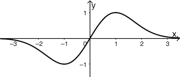 Abb. 1